Greek tragedies are caused by the conditions on unconditional loves. In particular, the fact that each character is obsessed with one and only one other character makes things complicated. As a result, there is no suitable matching of characters. Everyone gets disappointed. People blame each other. Eventually, things turn into chaos, for the greatest pleasure of the reader. Or, in the case of this extract from Community (great series BTW!), for the greatest pleaser of the viewer.
Now, suppose that the dean is organizing the prom. He wants to have as many couples as possible attending the prom. He thinks that by meddling in and choosing the couples himself he can do a better job than leaving it to the Greendale students. The list of guys includes Jeff, Abed, Troy, Pierce and Vaughn. The list of girls includes Britta, Annie and Shirley.
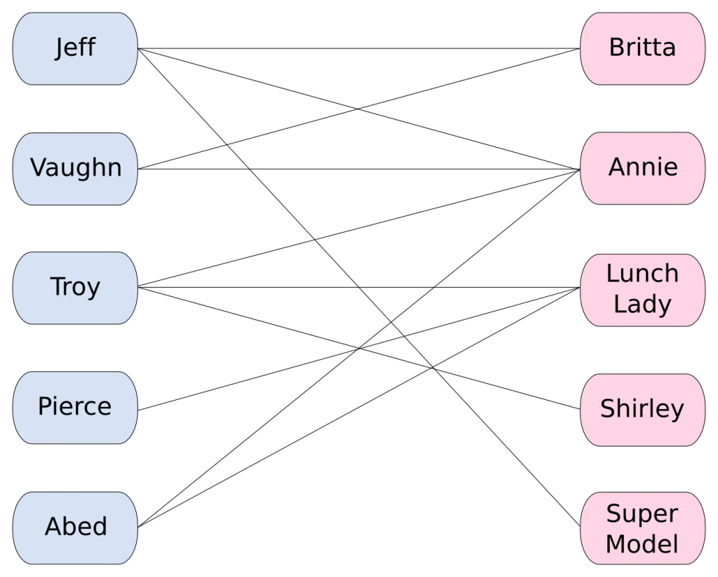
You’re right! Let’s add two more girls to match the number of guys: The lunch lady (the only girl that’d agree to go out with Pierce!) and a supermodel (that’d only agree to go out with Jeff!). The dean’s problem is to find as many matching as possible, with regards to the fact that if one person of a couple refuses to go out with the other, then the couple will not be attending the prom.
A usual way to model this problem is with the use of a graph (aka network). Each person will be represented by a point, aka node or vertex. A link between two nodes, called edge or line, will be drawn if the two persons represented by the nodes would both agree to go out with each other. The problem faced by the dean is actually a very classical problem in graph theory, called the maximum matching problem.
Maximum matching in a bipartite graph
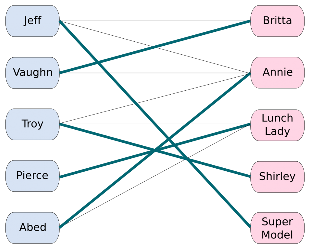
If the dean refuses to have homosexual couples attending the prom, then he may only consider edges linking a guy with a girl. Therefore, nodes can be classified in two categories such that two nodes of a same category are never linked. In graph theory, we say that each category is an independent set or a stable set. Graphs that can be divided into 2 stable sets like the one the dean has obtained here are called bipartite graphs. They are a very important class of graphs because of their specific structures that provide plenty of properties. Let’s draw the dean’s bipartite graph.
If we do the matching naively, we could associate each guy to the first girl that has not been matched yet. If we do that, we’ll match Jeff with Britta, Vaughn with Annie, Troy with the lunch lady… and that would be all as no match for Pierce nor Abed could have been found. The number of matching we would have ended up with would be 3. Not that great, right?
The method I have just described is called a greedy algorithm. Greedy algorithms are iterative algorithms, such that, at each step, we choose the next best step. However, because we don’t try to think the problem globally, greedy algorithms are not guaranteed to be optimal. Just like in this example. I have thought of a more advanced greedy algorithm that choose the guy with the smallest number of links and that match him with the linked girl with the smallest number of links. I couldn’t find an example in which this algorithm doesn’t provide the optimal result. Does this more advanced greedy algorithm always find the optimal result? I don’t know. But since it’d be a very quick algorithm and since no one mentions it, I guess it doesn’t. Please help me settle this.
Well, you’re right. I guess you can easily solve our problem here by mental deductions. But imagine that the list of guys and girls include every greendale student. This would be a much harder problem, wouldn’t it? Or, let’s be crazy, suppose the dean tried to invite every college student in the USA. Finding a solution wouldn’t be as easy and may not even be solvable with your single brain!
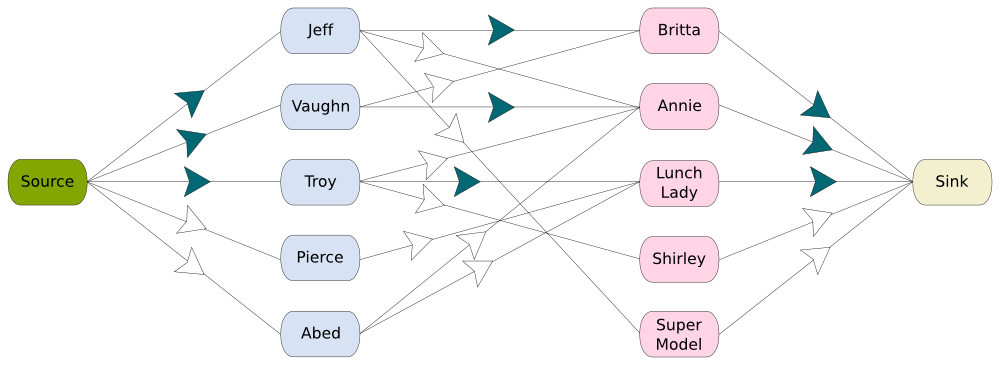
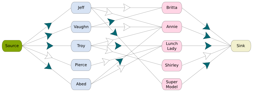
The most common way to solve this problem is by transforming it into a maximum flow problem. In order to do so, we add two nodes, called the source and the sink, on the left and on the right. We link the source to all guys, and the sink to all girls. We add a constraint to regular guy-girl edges: They have a capacity of 1. Now, we consider the problem of having a maximum flow from the source to the sink. The guy-girl edges that will be used for the maximum flow will form a maximum matching. Here is a figure of the flow corresponding to the solution obtained with the greedy algorithm.
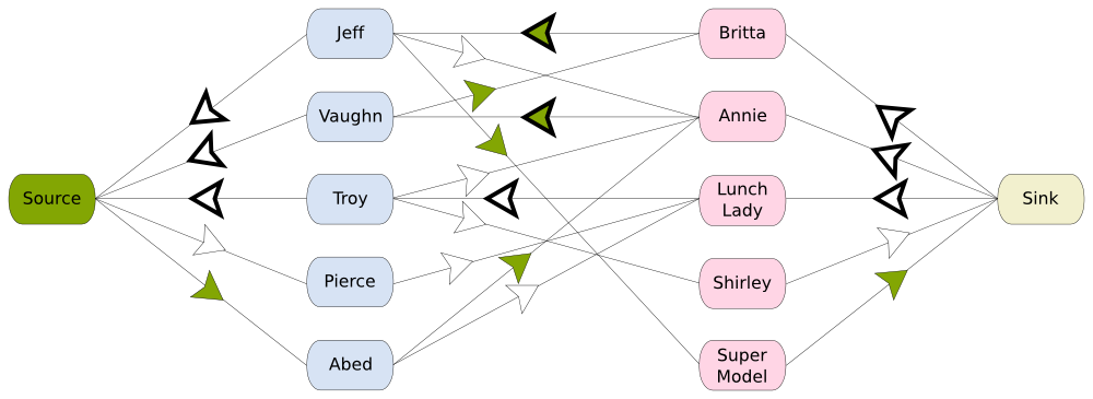
The maximum flow problem is a very classical problem with several other applications. It’d be interesting to have a more complete article on maximum flow problems and applications. Many algorithms have been developed to solve it. Most of them use the concept of the residual network. In order to build the residual network, we need to consider an admissible flow. Let’s consider the flow we’d obtain with the bad matching we had using the greedy algorithm. The residual network associated to the flow drawn above is obtained by inverting used arcs and give to the inverted arcs a capacity equal to the flow that was going through the arcs. The following picture is the obtained residual network, where inverted arcs have a bold arrow.
Let’s now apply the Ford-Fulkerson algorithm, invented in 1954. In the residual network, we search for a path from the source to the sink. This is a pretty easy thing to do. Just imagine you are in a maze and you have to find the exit. Just leave rocks on every intersection that indicate the paths you have already tried. If you find a dead end, come back to the last intersection with a path you haven’t tried and follow this unexplored path. Eventually, if there actually is a path towards the exit, you’ll find it. This method is a marker method. If you find a path from the source to the sink, add it to the flow we had. In blue is drawn such a path.
Don’t be scared. It’s very easy and intuitive. For instance, initially, there was no flow from the source to Abed. We add that to 1 flow from the source to Abed. This gives us… (come on, I know you get it)… 1 flow from the source to Abed. A little trickier now: we had a flow from Jeff to Britta, that we need to add to a flow from Britta to Jeff. This leads to… (come on, I know you can guess it)… no flow from Jeff to Britta nor from Britta to Jeff. Easy, right? Eventually, we end up we the following flow.
As you see, we have strictly improved our flow, hence our matching. Now, by iterating this process, we’ll improve our matching until there is no more path from the source to the sink in the residual network, in which case we’ll have reached optimality! Simple, right? It’s hard to believe that this algorithm is only 60 years old…
On the right is a figure of the maximum matching we’ll end up with.
Yes. There are several other algorithms that perform better. Mainly, they improve the way we choose the flow to be added in the residual network, by choosing simultaneously several paths (and by choosing them wisely!). The Hopcroft-Karp algorithm does precisely that, and it’s a particular case of Dinic’s algorithm. There is also an algorithm based on fast matrix multiplication. Although longer in practice, it has a better complexity for problems with a high ratio of edges per node, which means that it would perform better than other methods on super computers much more powerful than those we have today.
Obviously not. If there were no lunch lady, there would be no way to match Pierce with anyone. More generally, according to Hall’s theorem, there exists a perfect matching, that is, a way to have everybody matched, if and only if, for any subset of guys, their number is at most the number of girls they are linked to.
Maximum matching in bipartite graphs can be applied to any assignment problem. Replace guys by employees and girls by tasks. Edges are drawn if the employee is qualified to achieve the task. If employees can only handle one task at a time, then, as their employer, your best course of action is to choose a maximum matching.
You’re right. And in the marriage problem, this leads us to consider the guys’ and girls’ preferences. A simple way to do that is to associates attraction levels to edges. These levels could be numbers higher for couples that are more willing to go to the prom together. The problem we now face is to find a maximum weighted matching. In order to solve it, let’s add the missing edges between guys and girls and let’s give them a nil attraction level. Let’s start by finding a maximum matching. Then, observe than we can strictly improve it if and only if the residual network in which inverted arcs get the opposite of the arc attraction level contains a cycle with a cumulated positive attraction level. Repeating this will lead to a matching with the maximum attraction level.
The method we described is not the quickest known. The Hungarian algorithm performs better. There are great applications of this variant. Alternatives include solving linear programs. I’m not going to dwell on that though, as it’s not the best-known way to include the guys’ and girls’ preferences in the marriage problem…
Stable marriage problem
The more common way is to have guys sorting girls by how much they like them and vice-versa. We can now define what a stable marriage is. It occurs whenever the matching makes sure that no unmatched couple would rather be together than with their current match.
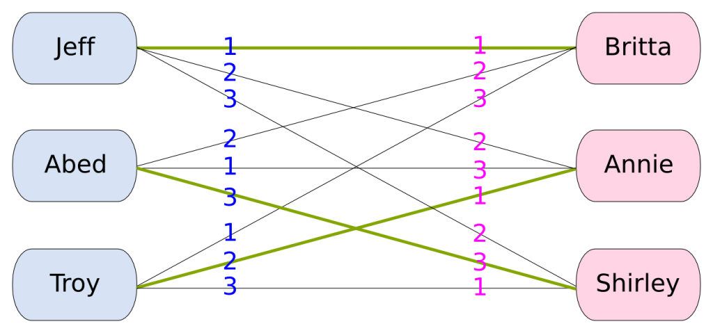
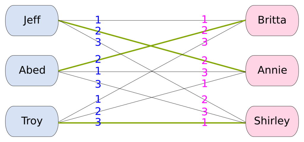
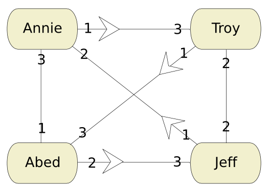
To avoid having a too complicated example, let’s kick the super model, the lunch lady, Vaughn and Pierce out of our problem (sorry Pierce!). The following figure shows each person’s preference.
The numbers on each person’s edges represent their ordering of the opposite sex. For instance, Jeff prefers Britta, then Annie and then Shirley. On the figure is drawn a matching. Considering this matching, Jeff would end up with Annie and Britta with Abed, despite Jeff and Britta preferring each other to Annie and Abed. Thus, the matching is not stable.
Yes. There is a method for just that! It was invented in 1962 and is known as the Gale-Shapley algorithm, and won Shapley a recent Nobel prize winner in economy! Let’s explain this iterative process. At each iteration, unengaged guys propose to the girl they prefer who has not turned them down yet, even if they are engaged to someone else. In our case, at the first iteration, Jeff and Troy propose to Britta, while Abed proposes to Annie. Then girls choose the guy they prefer among the one they are already engaged to and those who have just proposed to them (they don’t need to be faithful!). They are now engaged to that person. In our case, at the first iteration, Britta gets engaged to Jeff, while Annie is engaged to Abed. Then, we keep iterating until everyone is engaged (and then comes the weddings!).
At the second iteration, Troy is the only one who is not engaged. Britta has turned him down, so he’ll propose to his next favorite girl: Annie. Annie can now choose between her current fiancé, Abed, and the challenger Troy. She prefers Troy. Thus, she gets engaged to Troy while dumping Abed in the process.
At the third iteration, Abed proposes to his second favorite girl, Britta. Britta gets to choose between Jeff and Abed, but she prefers Jeff, hence she decides to stay with her fiancé. Abed gets dumped once again and is still not engaged. At the fourth iteration, he proposes to his third favorite girl, Shirley. Shirley is not engaged yet, so she accepts. Everyone is now matched. The algorithm finishes with the following stable marriage.
Yes I am. Here’s why. Girls that a guy prefer to the girl he’ll marry are those who have dumped him. Hence, those girls have found a better match. Therefore, there is no way that, to his wife, a guy prefers a girl that prefers him to her husband.
As a matter of fact, marriage stability is not really an optimality or a fairness criterium. Although, it has a bit of meritocracy as some guy who is always preferred to another and has the same taste will always end up with a better match. But if you are seeking for a more accurate sense of fairness, check my article on that topic.
Let’s remark that, in general, the stable marriage is not unique (even though in the example it is). It could be interesting to define a concept of optimality and to seek for an optimal stable marriage. But I haven’t found anything that does such a thing.
There is (at least) one interesting application. Imagine we allowed polygamy for girls only, limited to a certain number of lovers. That means that a girl could marry up to this number of guys. The problem becomes equivalent to affecting interns or residents to hospital, or students to classes or universities.
In order to have more applications of the marriage problem, we may also want to allow homosexual couples. Another way of understanding it is through the roommates problem. We have rooms of two persons only, and people don’t want to end up with anybody. Let’s see what happens.
Maximum matching in any graph
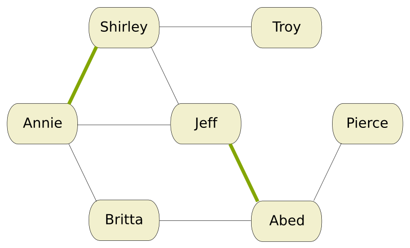
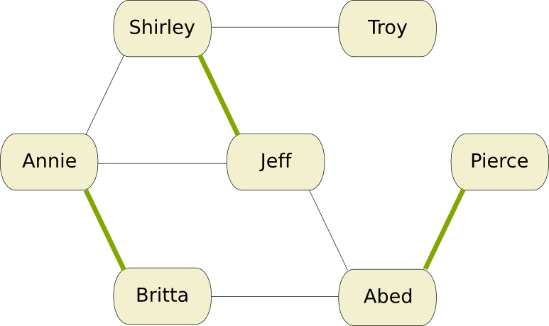
When we drop the guy-girl couple constraint, the graph we study is no longer bipartite. The marriage problem becomes a maximum matching problem in any graph. Let’s change our edges in our example to obtain a non-bipartite graph. Also we dropped a few nodes to obtain a more simple problem: we’ll restrict ourselves to the study group.
We have drawn a matching. This matching does not look maximum. We will search for an improvement of it using Edmond’s matching algorithm. We’ll call exposed node a node that is not in a matching. Edmond’s algorithm consists in finding an augmenting path, that is a path between two exposed nodes that alternates matching edges and non-matching edges. Then by switching the edges of the path from matching to non-matching and vice-versa, we’ll end up with a strict improvement of the matching. If no augmenting path is found, then we’ll have reached optimality.
Well, this is the more tricky part of the algorithm. Let’s consider the first exposed node alphabetically. This gives us Britta. We’ll build another graph that starts with her. She’s a linkable node. We’ll link her to her first neighbor in the initial graph chosen alphabetically. This gives us Abed. If this neighbor is an exposed node then our job here is done as the path from Britta to this exposed node is necessarily an augmenting path. Unfortunately, that is not the case. As a result, Abed is already matched, so he won’t be linkable and his match, Jeff, will be immediately added, linked to Abed. Abed’s match will be linkable.
We repeat the operation by choosing Britta’s alphabetically first linkable neighbor. This gives us Annie, who is linked to Shirley. Then, as Britta doesn’t have any neighbor to be added anymore, we move to the alphabetically next linkable node, which is Jeff. We choose Jeff’s alphabetically first linkable neighbor and we find… Shirley! This leads to a cycle that includes Britta, Abed, Jeff, Shirley and Annie. Here comes the trickiest part of the algorithm.
Whenever such a cycle is found we need to aggregate its nodes into a super node, in our initial graph. Nodes that were linked to one of the node of the cycle are now linked to the super node. We obtain the following graph.
We now repeat our algorithm by starting with Britta (actually, with the super node she has been included in) once again. Her alphabetically first neighbor is Pierce. Yet, Pierce is an exposed node. Therefore, the path from super Britta to Pierce is now an augmenting path. As a result, we can find an augmenting path from (not super) Britta to Pierce in the initial graph, that goes through nodes of super Britta. This path is the following: Britta, Annie, Shirley, Jeff, Abed, Pierce. Let’s switch edges of this path from matching to non-matching and vice-versa. We get the following matching.
Since the number of exposed nodes is now less than 2, this matching is now maximum. This solves the problem.
We surely can! This leads to the problem known as the stable roommates problem. Equivalently, it’s the problem of finding lab partner. Check this other extract from Community, where the study group (and the stranger Todd) try to find a maximum matching for biology 101. What they do is they each rank the others from favorite to least favorite. Then Abed makes a global ranking of people by popularity and matches the most popular and least popular people. This is not that good a system, as we consider the means of popularity, not individual preferences. What’s more it’s not a stable matching, as, and it’s shown in the episode, Jeff and Annie both prefer each other to their given partners.
What Abed should have done is applying Irving’s algorithm introduced in 1985 (that’s quite recent!). The existence of a stable matching here is not guaranteed. Irving’s algorithm tells us whether a stable matching exists, and, if it does, gives us one stable matching. Let’s illustrate the algorithm on our example. In order to make it simple, we’ll kick the unpopular out of the group: Todd, Britta, Shirley and Pierce (sorry Pierce!).
There are two phases of the algorithm. In the first phase, people propose and get proposals. If a person’s proposals have all been denied, he proposes to his favorite match that has not turned him down yet. If a person has several proposals, he turns down all but his favorite. Let’s consider an example and see what we get.
In this example, they all start by proposing to their favorite matches. Only Annie then has a choice to make, as she gets two proposals. She only keeps Jeff’s one, since she prefers Jeff to Abed. Then Abed has to propose to his second favorite match, Jeff. Jeff has no other proposal, so he accepts. Everyone now has agreed to a proposal and has a proposal that has been accepted. Phase one is over. If we eventually found someone whose proposals have all been rejected or someone who has never had any proposal, then that means that the stable roommates problem has no solution.
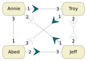
Suppose phase one was a success. Let’s move on to phase 2. In phase 2, we need to define for each person, his reachable next favorite partner, that is the person he prefers among those who he has not proposed to yet and that will accept his proposal because they prefer his to their current accepted proposals. The next favorite partners are represented by the dotted arrows in the following graph.
We are now going to look for a rotation that will improve the proposals. Let’s start with a node, say Jeff. Jeff is now associated with Annie. Let’s find each person’s favorite and who he will be replacing:
- Jeff’s next favorite is Troy, whose current proposal is from Annie.
- Annie’s next favorite is Jeff, whose current proposal is from Abed.
- Abed’s next favorite is Troy, whose current proposal is from Annie.
It does! Let’s have a look at the following graphical description of our reasoning.
We can make the changes, by replacing the current proposals of the rotation by the next favorite proposals. If we do that in our initial graph, then Annie would accept Jeff’s proposal and vice-versa, while Troy would accept Abed’s proposal and vice-versa. Thus, the algorithm finishes. The matching we’ve obtained is a stable matching!
Then there would be no actual solution. To be honest, I haven’t managed to fully understand what can happen with this algorithm. I’ve gone through the wikipedia page, but it’s not all clear. If you can help me, please do!
By the way, as a mechanism designer (that’s my PhD research topic), I have to think about the players’ incentives. If you have no knowledge of mechanism design, please read my article on that topic. When we’re applying these algorithms, would the characters from Community have incentives to lie about their preferences? In the stable marriage problem, it seems to me that being truthful is always optimal. In Abed’s method used in the episode of Community, they clearly do. As a matter of fact, Annie who knows she’ll be one of the most popular and will therefore be matched with the least popular should invert her preference list, hoping Shirley won’t end up least popular. In the roommates problem, it’s trickier to guess whether the players have incentives to lie or not. If I had to guess, I’d say they may have incentives to lie, but I need more thoughts on that matter. Obviously, your help is more than welcome here!
Let’s sum up
Love is a complicated issue. It always is. Matching people is a big challenge. If we don’t want to take into account their preferences, it becomes much easier and plenty of technics have been developed. However, trying to solve the problem when people have feelings and want them to be fulfilled makes everything much more complicated. Unfortunately, people are going to get hurt. Fortunately, this makes great stories.
We have shown several ways to deal with that issue. Yet, I’d like to highlight the fact that our criteria of stability are not the only way (and probably not the best way) to understand fairness or optimality of matchings. They define a good matching as no couple will both have incentives to flee their current matching. But anyone could end up being matched with his least favorite partner.



Thank you for all these beautiful graphs!