During the second world war, the soviet army was probably more efficient thanks to Leonid Kantorovich. In 1939, this mathematician and economist came up with a new mathematical technic to solve linear programs, hence improving plans of production at lower costs. In 1975, he became the only Nobel prize winner in Economy from the USSR. After the war, methods of linear programming kept secret got published, including the simplex method by the American mathematician George Dantzig and the duality theory by the Hungarian-American mathematician John von Neumann.
Applications in company daily planning rose, increasing efficiency thanks to linear programs. I don’t know to what extent linear programs have affected the outcome of the second world war, but it definitely has changed several markets, including electricity markets that uses it widely. Applications also include transport, supply chains, shift scheduling, telecommunications, yield management, assignment, set partitioning, set covering, advertisement. I’ve also heard of DNA analysis, and I personally use it for cake-cutting. If you know more applications, please tell me so I can update this list!
What’s more, linear programs become more and more useful as computers improve and more complicated problems can be solved. Several solvers have been developed, including CPLEX, Gurobi, Coin-OR and GLPK. They can solve linear programs with millions of variables in reasonable time.
You’re right. I should start with that. But as usual, I’ll do it with an example.
Let’s be smart robbers
Suppose we have just attacked a village and we want to steal as much as we can. There’s gold and dollar bills. But we only have one knapsack with a limited volume and we know we can’t take it all. So we’ll have to choose the volumes of each thing to steal. Also assume that we are not strong enough to carry too much weight (I do play sports but I don’t go to the gym, so I have a weak upper body…).

You face what is called a mathematical program or an optimization problem, which is the kind of problems addressed by operations research, also known as (very) applied mathematics. You need to maximize the value of your robbery by choosing volumes of gold and 1 dollar bills with constraints on total volume and total weight. One volume of gold is worth more than one volume of dollar bills but it’s also heavier.
The value of the robbery is called the objective function. It’s what we want to maximize or minimize. Volumes of gold and bills are called the variables. Mathematically, we usually write the mathematical program as follows.
$$\textrm{Maximise} \quad \textrm{Value(volume of gold, volume of bills)} \\\\
\textrm{Subject to} \quad \textrm{Total volume less than volume limit} \\
\textrm{} \qquad \qquad \quad \;\; \textrm{Total weight less than weight limit}.$$
Of course, we usually have complicated notations instead of words… But we’ll get to that!
So far, what we have here is a mathematical program. There are plenty of methods to solve a mathematical program but none of them can guarantee for sure that we find the solution in a reasonable time, especially if the number of variable is higher than 10. But in our case, we can write our mathematical program as a linear program.
And I’ll do it right now. A linear program is a mathematical program with a linear objective function and linear constraints.
In our case, the objective function is linear since, whenever you add a volume of any product, the total value increases by the value of that volume of that product. In other words, the value of the cumulated volumes of products is equal to the sum of each value of each volume of products. With formulas, that means that we can write the objective function in the following way:
$$\textrm{Value(volume of gold, volume of bills)} = \\
\textrm{} \qquad \qquad \qquad \quad \textrm{(value of 1 volume of gold)} \times \textrm{(volume of gold)} + \\
\textrm{} \qquad \qquad \qquad \quad \textrm{(value of 1 volume of bills)} \times \textrm{(volume of bills)}.$$
with constant multipliers for each variable.
I guess I should define what I mean by linear constraints. A linear constraint is a constraint that says that a linear function of variables must be higher, lesser or equal to a constant. Now, our first constraint says that the sum of all volumes must be less than some constant limit. This is obviously a linear constraint. Similarly, because the weight of volumes is the sum of weights of each volume, the total weight is also a linear function. Hence, the second constraint is also linear: our program is linear.
Almost. We forgot two constraints. So far volumes are assumed to be real numbers, but they actually need to be non-negatives. I mean stealing -1 litre of gold… that has no meaning. So we just need to add constraints that say that volumes are positive. Yet, these are linear constraint too! So our program is totally linear. Let’s write it again:
$$\textrm{Maximise} \quad \textrm{Value(volume of gold, volume of bills)} \\\\
\textrm{Subject to} \quad \textrm{Total Volume(volume of gold, volume of bills)} \leq \textrm{Volume Limit} \\
\textrm{} \qquad \qquad \quad \;\; \textrm{Total Weight(volume of gold, volume of bills)} \leq \textrm{Weight Limit} \\
\textrm{} \qquad \qquad \quad \;\; \textrm{(volume of gold)} \geq 0 \\
\textrm{} \qquad \qquad \quad \;\; \textrm{(volume of bills)} \geq 0.$$
In our problem, the mathematical program was already linear. However, in plenty of other cases, mathematicians actually modify their formulation of the problem or even make an approximation of their mathematical programs to obtain linear programs.
Because linear programs have a specific structure. This structure has been studied a lot. Plenty of results have been found, including optimization technics. Let’s talk about this structure.
Structure of linear programs
More than anything else, I believe that mathematics are about understanding structures. In linear programs, both the objective function and the constraints have nice structures. Let’s start with the constraints.
Our problem has two variables. We say that the vector of variables is of dimension 2. Now any two variables will not necessarily satisfy all the constraints, in which case we will say that the vector is infeasible. For instance, if the volume of gold is -1 and the volume of bills is 0, then the vector is infeasible because the constraint $\textrm{(volume of gold)} \geq 0$ is not satisfied. If our program had no constraints, any vector would be feasible, but constraints modify the feasible set.
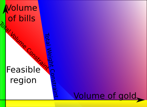
What’s interesting is how each constraint modify the feasible set. As a matter of fact, each inequality constraint divides the space into two areas, one for vectors satisfying the constraint, the other for vectors that don’t satisfy the constraint. Even better, this separation is a line (for higher dimensions the separation is a hyperplane). Eventually, when considering all constraints, the feasible set is a convex polygon (for higher dimensions, it is a polyhedron), as drawn in the following picture.
The red area is the area forbidden by the total volume constraint. The blue area is the area forbidden by the total weight constraint. Green and yellow areas are areas forbidden by non-negativity constraints. Hence, the feasible set is the white area. It’s a quadrilateral! That’s a simple mathematical object, right?
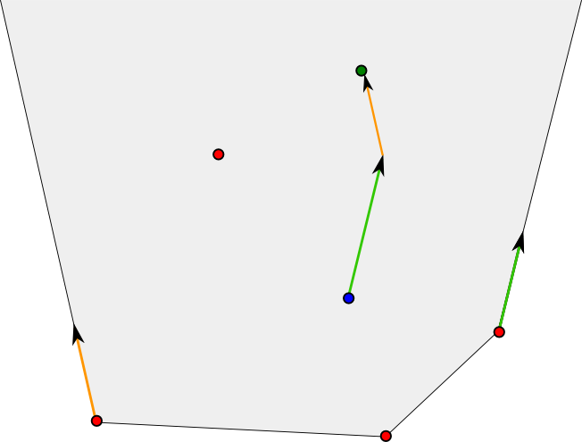
Well, we can define convex polyhedrons by saying they are the feasible sets of linear programs… But the interesting thing is more their equivalent definitions, given by Minkowski’s theorem in 1896. Convex polyhedrons can be defined with a finite set of points and a finite set of directions. They are all the points that can be reached by using a starting point in-between the finite set of points and by following some of the directions.
The image above displays a grey unbounded polyhedron. It can be obtained by choosing the red dots as the finite set of points and the the two vectors orange and green in the left and in the right. As you can see, any point of the polyhedron can be obtained by the process we described earlier. For instance, the green dot can be obtained by starting with the blue dot (that’s in-between the red dots) and by following directions given by the green and orange vectors.
In optimization problems, the directions are actually very simple to handle. They either lead to an infinite optimum for the objective function or have no effect. That’s why from now on, we’ll consider that there are none of these directions. In this case, convex polyhedrons are bounded convex polyhedrons. They are simply points in-between a finite set of points. Just like the following polyhedrons (which are the 5 platonic solids).

In the picture above are shown several bounded convex polyhedrons. You can see that they all have a finite number of extreme points and that all the other points inside the polyhedrons are points in-between the extreme points.
An extreme point of a convex polyhedron is a point that is not in-between two other points of the polyhedron. It might seem like I’m messing with you with all those sentences but I am not. As I said, a bounded convex polyhedron can be defined as all the points in-between a finite set of points, but this set of points is not necessarily the set of extreme points. Now, given a bounded convex polyhedron, we can define its set of extreme points. One interesting result is that a bounded convex polyhedron is the in-between points of its extreme points (read that carefully, it really is a theorem!). Basically, instead of describing bounded convex polyhedrons with linear constraints, we can equivalently describe them with extreme points.
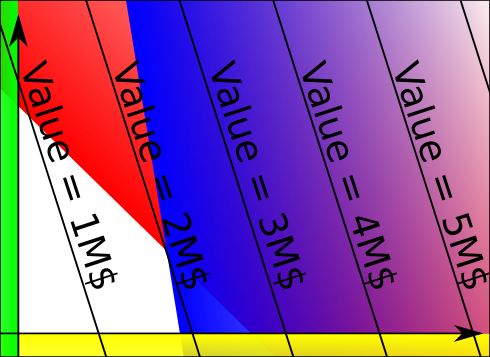
Sure. For each real number, we can consider the set of vectors for which the linear objective function’s value is that real number. This set of vectors is called the level set. What’s interesting is that level sets of linear functions are lines (hyperplanes in higher dimensions), just like linear inequality constraint’s separation. Let’s see what they look like in our problem:
When increasing the value of the linear objective function, the level sets move from left to right. Our mathematical program consists in finding the point of the feasible set that is on the level sets with the highest value. As you have guessed, our optimal value here is 2M$ \$ $.
Almost! As I said earlier, it’s possible that the optimal value is infinite because of asymptotic directions. It’s also possible that there exists no feasible vector, which means that the feasible set is empty and no vector can be considered as an optimum. Aside from these two cases, a theorem says that there always exists an extreme point that is one of the points that maximize the objective function. It’s possible that other points also maximize the objective function. Still, it means that if we know all the extreme points of our feasible set, we can easily solve our problem by testing them all! That’s a great structure, isn’t it?
And that’s not all! Any mathematical program can be associated with a dual program, which is another mathematical program that has interesting properties related to the initial mathematical program. In the case of linear programming, the dual program has even more interesting properties and many reasonings in this dual program enable major improvements (see my article on duality in linear programming).
Those which use the simplex method almost do that! Basically the simplex method moves from extreme points to strictly better extreme points. There’s a variant of it called the dual simplex that enables to travel via infeasible bases. Read my article on the simplex to know more about it. You can also learn the fundamental ideas with this extract from a talk I gave entitled a Trek through 20th Century Mathematics:
More recently, interior point methods have developed a lot. The idea is to add penalties for points close to the border of the feasible set and solve the optimization problem. As the penalties are reduced we get closer to the optimum. As computers improve, interior point methods show that they are more efficient to solve linear programs. However, many improvements of the simplex methods, in particular column generation, Bender’s decomposition and integer programming methods, are still much more efficient.
Let’s sum up
Mathematical programming is a difficult problem, and in some cases, solving problems with 10 variables can be awfully painful. However, if they have a linear structure, they can easily be solved even if they have millions of variables. Yet, in practice, only a few problems have the actual linear structure. But a lot of them can be considered as integer linear programs, which can be solved in reasonable time for thousands of variables. Find out more with my article on integer programming!
For particular integer linear programs, much research has been done and technics have been found to solve much bigger problems that could include with millions of variables. Still, many questions remain unanswered and technics to improve the simplex method for integer linear programs are currently being developed with more or less success, depending on the problem considered. That’s why the research on linear programming is still so important.
Besides, I strongly believe that the hardest part in optimization and operations research is the modeling part. I believe there are problems that have simply never been thought as integer linear programs and would gain a lot if modeled so. In fact, interior point methods have been proved to perform very well on convex quadratic problems. But the reason why they are not as popular as they should be is probably because modeling problems as programs for interior point methods is very tricky. Anyways, my point is that there is still a lot of research to do in linear programming.


I wonder if the careful “scaling” of math models like what is done with Finite Element Analysis, would provide a form of calculus based upon the non-dimensional models of scaling quantum causality. By introducing dimensional spaces, this seems to introduce limits to that may not apply to all dimensional spaces as might be involved with dark energy.
My spouse and I stumbled over here coming from a different website
and thought I might check things out. I like what I see so now i’m following you.
Look forward to exploring your web page repeatedly.