Is today’s financial world sustainable? How will it evolve? It’s hard to believe that one of scientists’ today’s best models to answer this question come from analysis originally made for biology, to mathematically describe Darwin’s paradigm! In fact, Darwin’s paradigm is good to make predictions and even better to explain why things are the way they are today. After all, for things to be what they are today, they have necessarily evolved into what they are today. These remarks have been the genesis of evolutionary game theory, which includes also the interactions of present things to predict their evolutions. This theory led to many applications in economics, environment and many more areas. I will explain it with the example of Rock Paper Scissors.
Rock Paper Scissors
Sure. Rock Paper Scissors is a two player game, in which each team can choose between three actions: Rock, Paper and Scissors. Rock beats Paper, Paper beats Scissors and Scissors beat Rock. The game can be summarized in the following figure, which displays the win of player 1 when it chooses the “row action”, while player 2 chooses the “column action”. Note that this is the classical representation of games in game theory, where the numbers of the array form a matrix called payment matrix.
Note that player 2 should also have his own matrix. These 2 matrices are enough to describe all the information of the game. In fact, any 2 player game with a finite set of actions for each player can be described with these 2 matrices, in which case we talk about bimatrix games. Playing each of this action only is called a pure strategy, as opposed to randomly choosing one of the action according to some random distribution, which is known as a mixed strategy.
Rock Paper Scissors has two important characteristics that we should highlight. First, it’s a nil-sum game, that is, whatever player 1 wins, player 2 loses it. Equivalently the payment matrices of the two players add up to the nil matrix. There are specific results in cases of nil-sum games, with, in particular, the minimax theorem, which says that the best player 1 can obtain if his strategy (which can be mixed) is known by player 2 is equal to the best player 2 can obtain if his strategy (which can also be mixed) is known by player 1. In our case, the best strategy of player 1 if his strategy is known by player 2 is the mixed strategy which corresponds to choosing randomly rock, paper or scissors, with a uniform distribution over each choice.
It can be deduced from this that this mixed strategy played by both players form a Nash Equilibrium, that is, a strategy profile from which none of the player has incentive to unilaterally deviate from. In other words, knowing that the other player will choose randomly rock, paper or scissors with uniform distribution, then there is no gain in not playing this mixed strategy.
The other important feature of Rock Paper Scissors is the fact that is a symmetric game. As a matter of fact, if we exchanged the ordering of player 1 and 2, the game would remain the same. Equivalently, the payment matrix of player 2 is the transposition of player 1’s. In such cases, it’s common to look for symmetrical strategy profiles, that is, situations where both players have the same strategy.
Nothing. And the reason is simple: It is not an evolutionary game. However, its resolution and understanding can be done by some reasoning on the populations of an evolutionary process. The classical example of evolutionary process associated to Rock Paper Scissors corresponds to the male populations of common side-blotched lizards. There are three sorts of them differentiated by the colors of their throats: either orange, blue or yellow. The orange-throated lizards have plenty of testosterone and therefore beat blue-throated lizards, which are smaller. However, blue-throated lizards are stronger than smaller yellow-throated lizards. However, these latter ones are of the same color as the females and can sneak around, as the orange-throated lizards don’t detect their presence. The blue-throated do detect them though, as they are more linked with females, and can therefore chase them away. Basically, orange beats blue, blue beats yellow and yellow beats orange. It sounds like Rock Paper Scissors, doesn’t it?

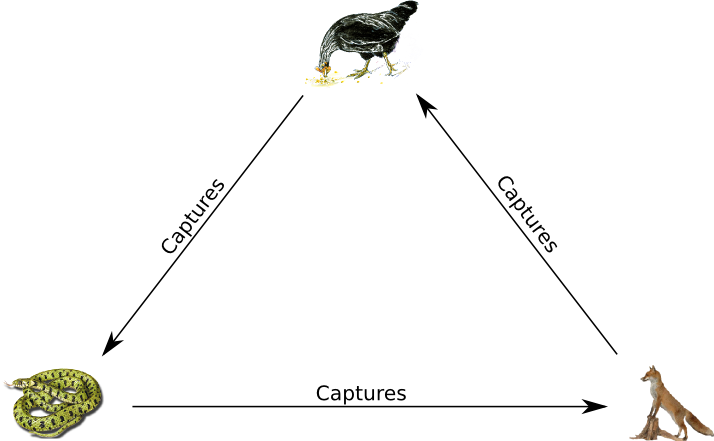
However this is not the population example we’re going to go with. When I was a child, I used to play a game called Hen-Fox-Viper (“Poule-Renard-Vipère” in French). We were about thirty kids divided into three teams. Each team corresponded to an animal. Hens were Vipers’ predators, Vipers were Foxes’, and Foxes were Hens’. Each predator had to capture all of its preys. The first team to have captured all of its preys was the winner, making its prey the loser. The third team was ranked second.
Now, I’m going to modify the rules to have them more suited to the analysis of Rock Paper Scissors with evolutionary game theory. We’ll suppose that whenever a predator captures one of its prey, it converts it into the predator’s species. For instance, if a Hen captures a Viper, then the caught Viper player become a Hen.
We match each kind of animal to one of the action, for instance, we match hens with rock, foxes with paper and vipers with scissors. To any population of remaining hens, foxes and vipers, we can associate the ratios of remaining hens, foxes and vipers over the entire population. These ratios can be associated with a mixed strategy, that is, if the ratio of hens is closed to 1, then the associated mixed strategy is to play rock very often. Now, the guess is that the ratios of remaining animals will converge, and that the limits correspond to a mixed strategy which is a Nash Equilibrium.
Well, in fact, the convergence is not guaranteed, it depends on the nature of the Nash Equilibrium… Let’s talk about game dynamics to sort this all out.
Replicator Dynamics
Let’s think about the dynamics of Hen-Fox-Viper. What would happen? How would the ratios of hens, foxes and vipers evolve in the future? Would they converge to some distribution? If it does, then we’ll be able to talk about an equilibrium of the nature, which, interestingly enough, will also be an Nash Equilibrium of the game. But we’ll get to that later.
The most common approach to game dynamics is based on Charles Darwin’s paradigm, which he introduced in 1851. According to him, the species that live today are those who have been more able to survive, because of statistical reasons. Indeed, others had trouble to reproduce themselves in sufficient numbers and were therefore doomed to disappearing. Mathematicians have captured this reasoning through an equation in the 1973 with the seminal work of John Maynard Smith and George R. Price, called the Replicator Equation.
No, I’m not going to show you a complicated equation. I’m going to show you an equation, and I’ll prove that it’s not complicated! This equation is a major equation in evolutionary game theory. Here it is:
[math]!\textrm{Variation of Population} = \textrm{Population} \times \textrm{Advantage of the Species}.[/math]
In biology, I should rather talk about the ability to reproduce itself. Or even more precisely, the average number of children per born animal. However, an interesting way to model the variation of population is to link this number directly with the current “advantage” of the population depending on its population, its environment and its interaction with the environment. Very often this “advantage” is defined as the fitness (or gain) of the species minus the average fitness of all species. OK, there is a second equation. Here it is:
[math]!\textrm{Advantage of the Species} = \textrm{Fitness of the Species} – \textrm{Average Fitness of all Species}.[/math]
Mainly, as we subtract the average fitness, if we initially had ratios of populations instead of populations, then the variables will remain ratios, as they will continue to sum up to 1. There are other ways to obtain similar dynamics based on reactions to the environment, including the generalized Lotka-Volterra equation or the Price equation. But they are equivalent to some Replicator dynamics formulation.
In our Hen-Fox-Viper example for instance, we could say that the “fitness” of Hen over Fox is -1, where as the “fitness” of Hen over Viper is 1. Finally, the “fitness” of a Hen against another Hen is 0. Eventually, this gives us the same array as for Rock Paper Scissors, which enables us to find results about Rock Paper Scissors by studying the dynamics of Hen-Fox-Viper.
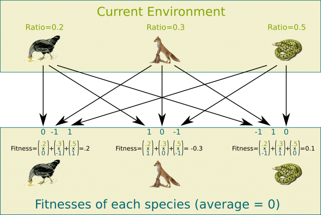
Now, suppose that the ratios of Hens, Foxes and Vipers are 0.2, 0.3 and 0.5. Then, the fitness of Hens in that environment will be the average of the fitnesses against each species, that is, (0.2 x 0) + (0.3 x (-1)) + (0.5 x 1) = 0.2. The following figure displays the species’ fitnesses.
It should have. In our case, it does have. Imagine that players were moving all in the field and there were randomly two players of any teams meeting each other. Suppose that one of the player is a Hen, then the probability that he is catching a prey is the probability that the other player is a Viper, which is equal to the ratio of Viper, that is, .5. But the probability that he is being caught is the probability that the other player is a Fox, that is, .3. Therefore, the expected increase of the population of Hens in this meeting where one of the player is a hen is equal to .5-.3=.2. Thus, this dynamics actually describes well the actual dynamics of the game, in the case where meetings were uniformly random.
Well, the average fitness is the gain of the mixed strategy composed of the environment against the environment, which is the mixed strategy itself. Thus, the average fitness is necessarily the gain of a mixed strategy against itself. Yet, since the game is a nil-sum game, this average gain must be the opposite of the gain of the opponent mixed strategy. Because the game is also symmetric, these two gains must be equal. Zero is the only number which is equal to its opposite, thus the average fitness is necessarily equal to zero.
As a result, the advantages of Hens, Foxes and Vipers are respectively .2, -.3 and .1, which means that the variations of their populations according to the Replicator Equation are respectively .2x.2=.04, .3x(-.3)=-.09 and .5x.1=.05. This will imply new ratios of population, then new fitnesses. This will in turn give new variations of ratios of population, and so on. What we are describing here is a classical differential equation systems.
I’m not going to do that. Differential equations are a very interesting field and very important in evolutionary games. But there is already so much to talk about here. If you know about differential equations, please don’t hesitate to write about them.
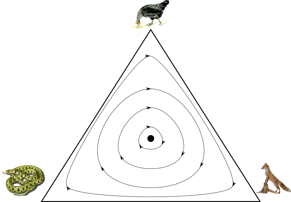
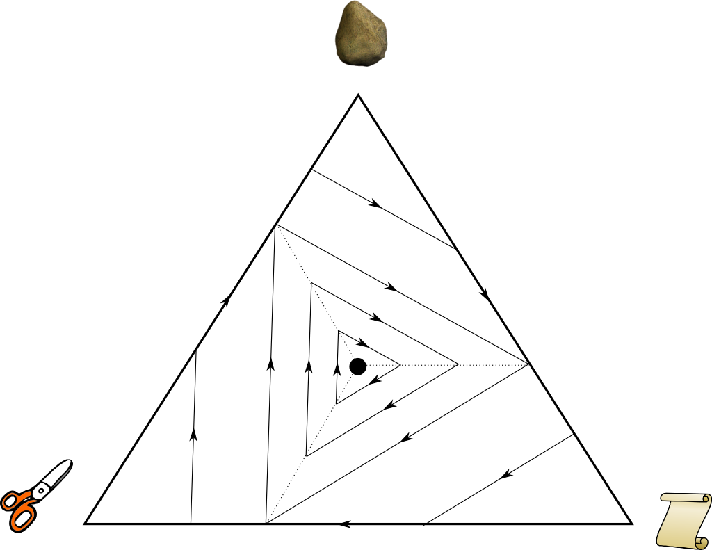
Basically, what you need to know here is that there are mathematical tools to solve or to approximately solve differential equations. In our case, the equations are linear, which makes them relatively easy to solve. Now, one way of representing the dynamics of the population is by drawing the trajectory in a triangle. Each summit of the triangle corresponds to a species being predominant. Each point inside the triangle is a barycentre of the summit, with weights that correspond to the ratios of population. Basically the closer a point is to a particular species, the higher is the ratio of population of that species.
The following figure displays the trajectories we have depending on the starting point. Let’s note that equations lead to observing that the product of ratios of populations must be constant, thus trajectories must follow level curves of the product of ratios.
This dynamics is called the Replicator Dynamics.
Evolutionarily Stable Strategy (ESS)
Indeed, all of the paths are cycles. Thus, there will be no convergence in this case. However, one thing we can notice is that if we start close to the black dot, which is the center point of the game and corresponds to equal ratios of each species, we will always remain close to the center point. In such a case, we say that the black dot is a stable point of the dynamics. Notice that the black dot is the Nash Equilibrium we mentioned earlier.
Almost! It’s the case for any stable point strictly inside the triangle. As a matter of fact, if a point is a stable point, then the variations of ratios must be nil. As a result, because this variation is proportional to the advantage of species, and since populations are strictly positive inside the triangle, the fitness of each species must be equal to the average fitness of all species. Therefore, no matter what mixed strategy of the triangle we play, the gain will be the same of the average gain of all species, which is the gain of the mixed strategy of the stable point against itself. Therefore, there is no reason to deviate from the mixed strategy of stable point, which means that the stable point is a Nash Equilibrium.
There can actually be a convergence towards an interior stable point. Let’s see how in an example. Suppose now that, whenever a predator capture a prey, not only does he convert his prey but he also gets a new partner (as if he reproduced with the converted prey). In such a case, each species would grow better if its environment contains both its prey and predator than if was all alone. This gives us the following matrix of gains.
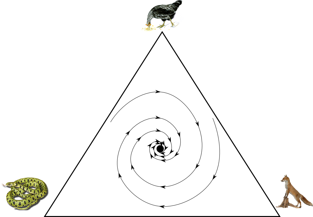
The game is still symmetric, which means that the gain matrix of player 2 is the transpose of this gain matrix. However, it’s no longer a nil-sum game. As a result, the average fitness is no longer equal to 0. It actually depends on the ratios of population. Anyways, we can still draw the dynamics of the ratios, which would give something that looks like the following:
As you can see all paths from the interior of the triangle converge to the central black dot. We say that the black dot is not only stable, but also asymptotically stable, that is, if we start the dynamics close to it, we will ultimately converge to it. Just like before, we can show that any stable point is a Nash Equilibrium.
However, the nature of this Nash Equilibrium is different from earlier. Indeed, in this case, not only do we remain close to the Nash Equilibrium, but we actually converge to it. This has led to the definition of another concept: The black dot here is an Evolutionarily Stable Strategy (ESS).
Almost. Actually, an ESS is a strategy such that, for any other strategy close to the ESS, the ESS is a better strategy against the other strategy than the other strategy against itself. Thus, even if the strategies slightly deviate from the ESS, the ESS will remain the best-reply, which makes it an asymptotically stable Nash Equilibrium. As a result, ESS are asymptotically stable (a accurate proof would require the introduction of a Lyapunov function) but I’m not sure that in the general case an asymptotically stable point is necessarily an ESS. I feel like it might be the case for a finite set of action, but maybe not in the general case.
For population dynamics, we can interprete an ESS by saying that if the ratios of population match an ESS, then any mutation of populations, which leads to a deviation from the ESS, will result in the disappearing of this deviation. We say that mutations cannot invade the populations.
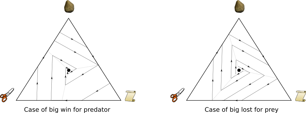
Similarly, we can define an anti-ESS, which corresponds to repulsive point. Whenever we start close to a repulsive point, the dynamics flees away from the repulsive point. Let’s get back to Hen-Fox-Viper and change the rule to create an anti-ESS. Now, whenever a predator catches a prey, the prey is converted and a prey’s lover dies, hence making the prey’s population decrease by 2. This gives us the following payment matrix and the following dynamics.
As we can see on the figure, the dynamics of the population leads to te disappearing of two of the three species, unless we start exactly at the anti-ESS point, which is a Nash Equilibrium. In fact, an anti-ESS can not be observed in real population ratios, as it is unstable. A mutation of the ratios would ineluctably lead to a dynamics that flee the anti-ESS. For instance, for the side-blotched lizards, we can say that a good modeling needs to generate an Nash Equilibrium in the interior of the triangle which is not an ESS, as it would mean that two of the three species would end up disappearing. Therefore, the concept of ESS is even more relevant than Nash Equilibrium, at least in dynamical games.
Best-Reply Dynamics
The replicator dynamics is an interesting dynamics that translates mathematically the ideas of Charles Darwin. However, it’s not the only dynamics we can think of. In fact, the first idea of dynamics in game theory comes from George W. Brown in 1951, much before the concept of the Replicator dynamics. In his idea called fictitious play, we imagine a sequence of games, in which each player reacts to the mixture of past strategies played by the opponents. Although this ideal is sequential, we can extend this concept to continuous time dynamics. Given the mixture of past strategies of the opponent, there exists a set of best-reply strategies to this mixture. The idea of continuous best-reply dynamics is to have the strategies of each player varying towards the best-reply strategy. It’s a great way to model the behaviors of smart players who react to their environment by reasoning. This is captured in the following equation:
[math]!\textrm{Variation of Strategy Mixture} = \textrm{Best-Reply Strategy} – \textrm{Current Strategy Mixture}.[/math]
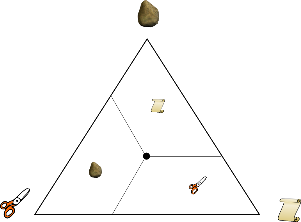
Let’s apply this to the classical Rock Paper Scissors. It can be shown that if Scissors is a better-reply than Paper if and only if the opponent plays Paper and Scissors more often than Rock. As a result, we can divide the triangle of mixed strategies into three areas in which there is only one best-reply strategy, as follows.
Now, more precisly concerning the dynamic, in each of the tree areas, the best-reply is not a mixture, thus, one of the ratio will increase while the two other ratios will decrease at the same rate. Graphically this means that the direction of variation is perpendicular to the axis linking the two pure strategies which ratios will decrease. This gives us the following dynamics.
Just like earlier, the Nash Equilibrium of the classical Rock Paper Scissors is a stable point of the dynamic here.
Well, the difference will be the division of the triangle into areas with same best-reply strategies. You could do the calculation to see what are the conditions for Paper to be better than Scissors, it’s a little bit of addition, nothing complicated, but not very interesting to explain here. This gives us the following dynamics.
Indeed. I have had the chance to attend a presentation by Josef Hofbauer, one of the top scientist in this field. He presented six different dynamics and showed that for almost all of them, the ESS was asymptotically stable, where as, for all of them, the anti-ESS is repulsive.
That’s a great question. In fact, Josef Hofbauer proved in his presentation that there does not exist a dynamics such that all anti-ESS are stable. In particular, he presented a sequence of ESS such that for any dynamics, there exists a rank such that ESS beyond this rank are all repulsive. My understanding of this is not good enough and it’s a bit long to present here, but it’s a very nice proof so I’ll try to write something about it some day! If you know it, please write about it!
Now, best-reply dynamics are often considered as myopic dynamics. It corresponds to choosing the best reply to past actions of the opponents, but it doesn’t take into account the future reactions of the opponents, nor possible evolutions of the environment. In order to take into account the future, evolutionary games consider the strategies taken by players at each time of the future. Their gain is usually modeled by a time exponentially-discounted sum of gains at each time of the future. Obviously this makes equations much more complicated, but once again, there are mathematical tools to handle this. In particular, control theory and viability theory enable resolutions in certain cases. There is a lot to say on those theories and I don’t have a great understanding of them. If you know about them, please write an article!
Let’s sum up
Evolutionary game theory is also appealing to sociologist. I don’t really how they interpret it, but I definitely understand the interest for it. Indeed, the replicator equation can also describe human behaviors. Not only does it greatly explain why some civilisation may disappear, but it’s also a modeling of the fact that whenever something seems appealing, the number of people who adapts it will increase. If the Internet makes developers rich, there is no doubt that more and more people will learn computer science, hence increasing the community of developers.
We have presented to two ways of explaining evolutions. The first one, the replicator dynamics, follows Darwin’s principles, and can be summed up by saying that misfit populations are doomed to disappear, and can therefore not be observed today. The second one, the best-reply dynamics (and extensions for gain optimization) involves the cleverness of species and their willingness to adapt themselves to survive and prosper. Any of the two dynamics imply evolutionary stable strategies. In societies, they probably both apply. This explains why developing start-ups are necessarily run by risk-lover people: You need to be this sort of person to be willing to launch a start-up, and a start-up also needs such a person for it to be fit to develop.
There are other dynamics though. Let’s have a look at Facebook. Hundreds of millions of people have registered and use it. It seems that the reason why people use Facebook is not because it’s a smart decision, nor is not using Facebook making people misfit. Rather, people connect to Facebook because their friends are connected. They are influenced. They are transformed by their surroundings into Facebook-connected people. I know that professor Asu Ozdaglar from MIT has worked on such dynamics, called opinion dynamics.


