While the 2014 World Cup in Brazil is approaching, controversy has been raised about the FIFA ranking which plays a central role in the drawing of the first stage groups. In particular, it’s puzzling to see that this ranking (in October 2014) features Columbia and Belgium at 4th and 5th position, while world-cup winners Brazil and France are 11th and 21st… Does this ranking even make sense?
I’m not going to explain it, but I can tell you it involves a lot of parameters! And that’s bad, as many of these seem arbitrary, such as the one describing the weakness of the opposition, or the weighting of the different confederations!
In this article, I’m going to present an old work I did 7 years ago with Professor Franck Taïeb on a modeling of football games. I then applied this modeling to simulate the 2006 world cup, with surprisingly good results! And as we’ll see, this modeling leads to a more natural way of computing the actual strengths and weaknesses of national football teams!
This article covers all major steps of modelings in general. Thus, I believe it to be interesting even though you’re not that much into sports. Note that this modeling would work for similar sports, like handball, basketball, American football, hockey…
Parameterized Probabilistic Model
Let’s imagine that the final of the 2014 world cup opposes Brazil to Argentina.
This game can be regarded as a random event. In particular, the numbers of goals scored by each team are assumed to be random variables. The first important step of our modeling is to choose a probabilistic law to describe this random variable.
A simple way of modeling the number of goals Brazil scores is to divide the 90 minutes of the games into 6 periods of 15 minutes. At each period, there is a certain probability p that Brazil scores. Assuming that Brazil scores at most one goal in each period, the number of goals Brazil scores in one period follows a Bernoulli distribution. This means that it equals 0 or 1, with a fixed probability that it equals 1.
We’ll get rid of this assumption in a few lines! Let’s stick with this right now. Let’s also suppose that the probability of Brazil scoring is the same for all periods and that every two periods are independent from each other.
I know! But for simplicity and computations, we won’t be able to work things out without this assumption. Denote p this probability of scoring in a given period.
The total number of goals Brazil scores is the sum of the numbers of goals in all 6 periods. Thus, it is the sum of 6 independent and identically distributed Bernoulli variables which equal 1 with probability $p$.
Before computing this, let’s calculate the probability of Brazil scoring a goal in the 4th and 6th periods only. This event corresponds to the following configuration:
To obtain this configuration, not only does Brazil need to score in the 4th and 6th periods, but it’s also necessary that Brazil doesn’t score in other periods. Because we have assumed that all periods are identically distributed and independent, the probability of the configuration is thus the product of the probabilities that each period ends up accordingly to the configuration. This product equals $(1-p)(1-p)(1-p)p(1-p)p=p^2(1-p)^4$.
What we have seen so far corresponds to one configuration where Brazil scores twice. To compute the probability of Brazil scoring twice, we simply need to add up all probabilities of all configurations where Brazil scores twice. The following figure lists them all:
In our case, there are 15 configurations. (Try to prove it!)
The number of configuration is equal to the number of ways to choose 2 scoring periods out of 6. This number is called the binomial coefficient, and is denoted ${6 \choose 2}$. You can compute it by googling 6 choose 2. On calculators, you have to spot the button nCr.
More generally, if there are $n$ periods, then the number of configurations corresponding to Brazil scoring $k$ goals equals ${n \choose k}$. Since a particular configuration corresponds to scoring in $k$ periods and of not scoring in the other $n-k$ periods, we finally obtain the following formula, known as the binomial law:
Great remark! Indeed, a weird assumption we made was that only one goal could be scored in each period. A simple way to overcome this is simply to divide the length of the game in many more periods. But, as we increase the number of periods we have to keep track of the fact that the average number of goals scored in the whole game shouldn’t get modified. This average number of goals in the whole game equals the number $n$ of periods multiplied by the probability $p$ of scoring in one period.
The bigger the better, right?
Let’s take the biggest possible value for $n$, which is… infinite! Like often, things become much simpler once we get the parameter goes to infinity. The binomial law then converges towards a Poisson law, named after French mathematician Siméon-Denis Poisson. This law now depends on one single parameter commonly denoted $λ$ (lambda). This $λ$ equals the average number of goals.
You can check it out, but let’s not dwell on too much on this technical detail. Rather, now that we have a parameterized probabilistic model, let’s move on to the next phase.
Maximum Likelihood Estimation
The next phase is to determine the right parameters of the model. In other words, how can we define the parameter of the Poisson law which describes the numbers of goals Brazil will score against Argentina?
Yes! Thus, for every team, we introduce two variables. One for attack skills, and another for defense weaknesses. The average number of goals Brazil scores against Argentina will then be the product of Brazil’s attack skill and Argentina’s defense weakness.
Sort of. Except now, there are relations between the parameters of different games. This is essential for us to go further. This also means that we need to include all parameters of all teams in our model. The following figures displays all parameters we need to estimate to define the probabilistic model:
We are going to use past results to estimate the parameters. There are several ways to retrieve parameters from past results. In our case, we are going to use a technic called maximum likelihood estimation (MLE).
If we fix the values of parameters, then the probabilistic model is well-defined. Thus, we can then compute the probability of the past results. This probability is called the likelihood. More precisely, the likelihood is the mapping of values of parameters with the induced probability of past results. The MLE then consists in choosing the parameters which maximize the likelihood. In other words, the parameters which make past results the most likely possible.
Yes. To do so, we assume that games are independent. The likelihood is thus the product of the probabilities of each past game. Now, to then maximize the likelihood, we need to calculate the partial derivatives of the likelihood with regards to parameters. This is much easier to do for sums rather than products. Thus, we usually rather maximize the logarithm of the likelihood, which I’ll call the log-likelihood. We end up with the following equations:
The variables games count the number of games involving the two teams. Note that there’s one equation for each parameter. Thus, there are twice as many equations as the number of teams.
Not exactly. The parameters must satisfy these equations to maximize likelihood. However, they might satisfy these equations without maximizing likelihood. Mathematically, we say that satisfying these equations is necessary but not sufficient.
Computation of Parameters
Before actually computing the parameters, let’s notice that we could multiply all attack skills by 2 and divide all defense weaknesses by 2, and everything would remain the same. This homogeneity implies that there cannot be unicity of the solution. This usually causes a lot of computational issues. Fortunately, we can fix one parameter to 1, say Brazil’s attack skill. Then we can optimize over the rest of the parameters. This reduces the problem to a much more classical one.
The simplest approach is to proceed with an iterative algorithm. We start with certain values of the parameters. Then, at each iteration, we use the first kind of equations to update all attack skills but Brazil’s, given the defense weaknesses defined so far. Then, we update all defense weaknesses with the second kind of equations, given all attack skills.
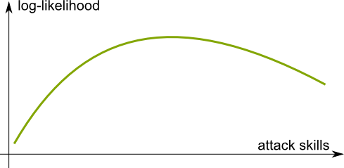
Hummm… Let’s notice the concavity of the mapping of attack skills with the log-likelihood. Similarly, when attack skills are fixed, the mapping of defense weaknesses with the log-likelihood is concave too.
Concavity corresponds to the shape of the curve of the function. A function is concave if the curve looks like the mouth of an unhappy person.
The great thing about concave functions is that a point maximizes the function if and only if the derivative at this point is nil. Thus, each of the two steps of iterations is a maximization of the likelihood.
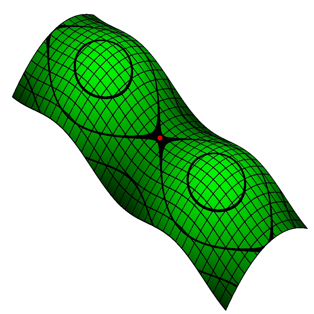
Unfortunately, no. Although the log-likelihood is concave with regards to attack skills, and with regards to defensive weaknesses, it is not concave with regards to both. As a result, it may have a shape like the surface on the right taken from Wikipedia. In both horizontal and vertical directions, the surface is concave. But it is not in diagonal directions. This means that the convergence and the optimality of parameters are difficult to guarantee in the general case.
This is great question. Let me rephrase it. Isn’t there some reasonable sufficient condition which would guarantee the convergence of the iterative algorithm towards the optimum? It’s typically the sort of questions I’m trying to answer in my current research with other algorithms!
So first, let’s give a sufficient condition to the existence of an optimum. Indeed, this is far from guaranteed. Imagine we compared European teams and South American ones, based on results which do not include any game between a European and a South American one. We would not be able to compare the levels of teams of different continents. This could mean that there is no optimal choice of parameters.
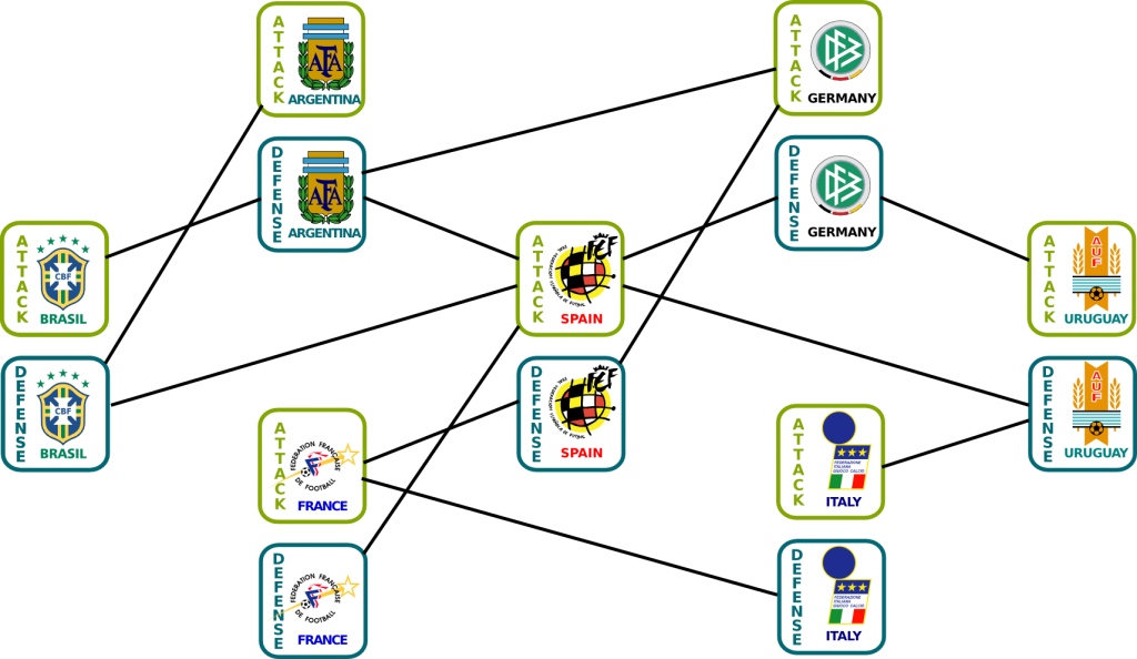
Mathematically, this corresponds to a sufficient condition which can be stated as follows. Let’s consider the graph of parameters. We add links between an attack skill of a first team and a defense weakness of a second team if the first team has ever scored against the second in the past results considered. For instance, we could obtain the following figure:
If any two variables are connected by a path, then we say that the graph is connected. This condition of connectedness is sufficient for the existence of optimal parameters.
No, it doesn’t. Unfortunately, providing a sufficient condition is more complex. The simplest sufficient condition for the convergence I have come up with is the injectivity of the log-likelihood restricted to points where the gradient is nil (this is already hard to prove!). But this sufficient condition doesn’t guarantee the convergence towards the optimum.
Let me finish this mathematical analysis with a statistical remark.
Yes, because what we are doing here – estimating parameters based on past results – is a typical statistical problem. In particular, it’s necessary to test the rightfulness of the estimation of parameters. A common test consists in giving values to the parameters. We then simulate the results, and use these results to estimate the parameters. We then compare the estimated parameters with the initial parameters. If, in average, they match, the statistical process is called unbiased. If, as the number of simulated games goes to infinite, the estimated parameters always match the initial parameters, the statistical process is called consistent.
Mathematically, it seems very hard to prove. However, I have done simulations to have a hint at the answer. The estimators appear to be biased for limited numbers of games. But they also seem to be consistent.
No. To go further, we’d need test our model. Learn more with my article on hypothesis testing.
Simulations of 2006 World Cup
Now, let’s get to the fun part. I used all results of all games which had been played two years before the 2006 world cup to compute the skills of all teams. And then, slightly before the 2006 world cup, I simulated the world cup, over and over, with these computed skills.
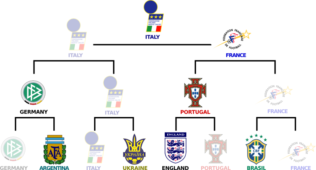
And here are the results! The percentages in the figure below represent the frequency at which each team won the world cup in my simulations:
Well, we can compare them with what actually happened… Italy won the world cup (at my greatest disappointment) and France finished second (I still remember Zidane’s header at 111 minutes saved by Buffon… Why is Buffon so good???). Germany and Portugal lost in semi-final. The rest of the standings can be read in the following figure:
I know! The first three teams of the simulations all made it to the semi-finals! Plus, 7 of the last 8 teams are in the top 10 of the simulations. Even more impressive, in the top 16 of the simulations are 14 of the last 16 teams!
Well, I strongly feel that the results are misleadingly right. The fact is that the 2006 World Cup had very few surprises, and that’s why the simulations match what eventually occurred.
One big surprise to me is how big the probability of winning is for underdogs. By underdogs, I mean teams which are not in the top 8, as acknowledged by specialists. Teams like Switzerland, Poland, Mexico, Ukraine, and so on, are often considered underdogs. The probability of an underdog winning sums up to 21.9%. This means that one out of 5 world cup should crown an underdog. However, World Cup finals have only included big teams. This suggests that big teams might have this ability to be at their best when it matters. Or, rather, that they are not at their best in the friendly and qualifying games before the actual competition.
Let’s Conclude
What I’ve presented here is an application of a more general method to modelize phenomena. Namely, we first define a parameterized probabilistic model. Then, we estimate these parameters based on past observations. The Maximum Likelihood Estimation is one way of doing this. It involves an optimization problem which generally requires gradient-based technics. The computed parameters can then be used to simulate future events. At this point, there are two important elements to test. On one hand, we need to verify that the optimization problem has been solved optimally. On the other hand, we shall test bias and consistency of the estimation of parameters.
Hehe… Two years later, in 2008, with 6 other students, I studied how bookmakers set wagers to maximize their profits. What mostly comes out of this study is that they have to make sure that bookmakers’ wagers all match. In fact, they cannot afford to differ by much. Indeed, otherwise, there would be a way for players to bet so that their win will be positive for sure. Players should then bet an infinite amount of money. This means that the bookmaker’s revenue would have an infinite variance… which is never good… Overall, I don’t think that the model is good enough to make money out of it.
One major advantage of this modeling is that there is no need to introduce arbitrary parameters to describe the weakness of the opposition, nor the region of Earth where this is played, as is done in the current FIFA ranking. Another relevant point of this modeling is that it makes a difference between a 6-0 win and 1-0 win, which the current FIFA ranking does not. However, we haven’t obtained a ranking of teams. Rather, each team is represented by an attacking strength $a$ and a defending strength $d$. But a team $i$ is then more likely to win against $j$ if its expectation of scoring is greater. This corresponds mathematically to $a_i d_j > a_j d_i$, and can be rewritten as $a_i/d_i > a_j/d_j$. Thus, the ratios $a/d$ is a good way of ranking the teams. Overall, yes, I believe the approach of this article is more relevant to rank football teams!
To improve the model, we need to identify key factors which strongly affect the outcomes of games and have not been taken into account. For instance, we have assumed games independent. Football amateurs have probably noticed that this excludes the concept of confidence of a team. The better a team is doing, the more likely it is to win its next game. Conversely, a team which is doing bad (and is in crisis), is less likely to be doing well in the next game. This idea can be modeled by the powerful (but complex) concept of Markov chains.
Other improvements could involve taking into account the playing home factor or the major player missing one. But keep in mind that the more parameters you introduce, the less relevant the computed parameters will be. Thus, for instance, to model major player missing, it’s unreasonable to model each player individually. Rather, you could think of a model where each player has an influence on his team (which could be related, for instance, to the percentage of time he plays). We could then map this influence with some drop in the team’s skills when the player is missing.
This research was done in my second preparatory year in France, as the TIPE (Travail d’Initiative Personnelle Encadrée). I then presented it at the entrance exams of Engineer Grandes Écoles (where they loved it and gave me 19/20) and of the prestigious École Normale Supérieure (where they didn’t and gave me 6/20).


