Santa Routing and Heuristics in Operations Research

As a child, I always wondered how Santa Claus could visit all children of the world overnight. I now know that he must have a very optimized route plan. And this tells me one thing: Santa Claus is a math genius!

In the last decades, similar problems called vehicle routing problems have become crucial for many companies, like Fedex and UPS. And these are so difficult, that companies asked help from applied mathematicians! Since then, applied mathematicians have enjoyed the beautifully combinatorial structure of these problems, as well as the millions of dollars companies have been willing to pay for answers! Let’s see what these mathematicians have come up with! This will draw a global picture of the world of operations research, which, more generally, aims at solving complex combinatorial industrial problems through mathematics.

Santa’s Vehicle Routing Problem

If there were no constraint on Santa Claus’ journey, the visiting-all-children problem would be a Traveling Salesman Problem (TSP): It would consist in searching for the shortest path visiting all cities and coming back to the original point. This class of problem has become iconic in the theory of computation, as it was proved to be very hard to solved!

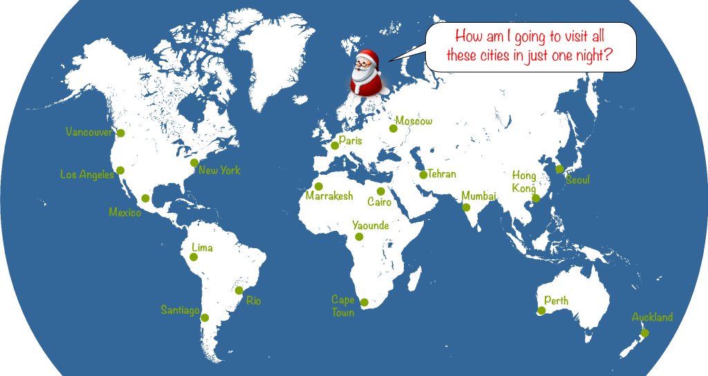
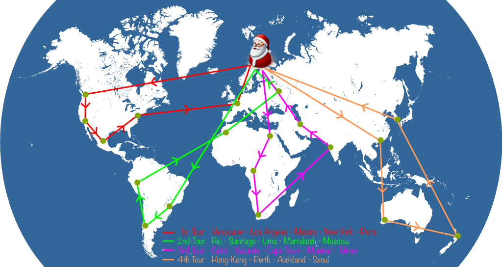
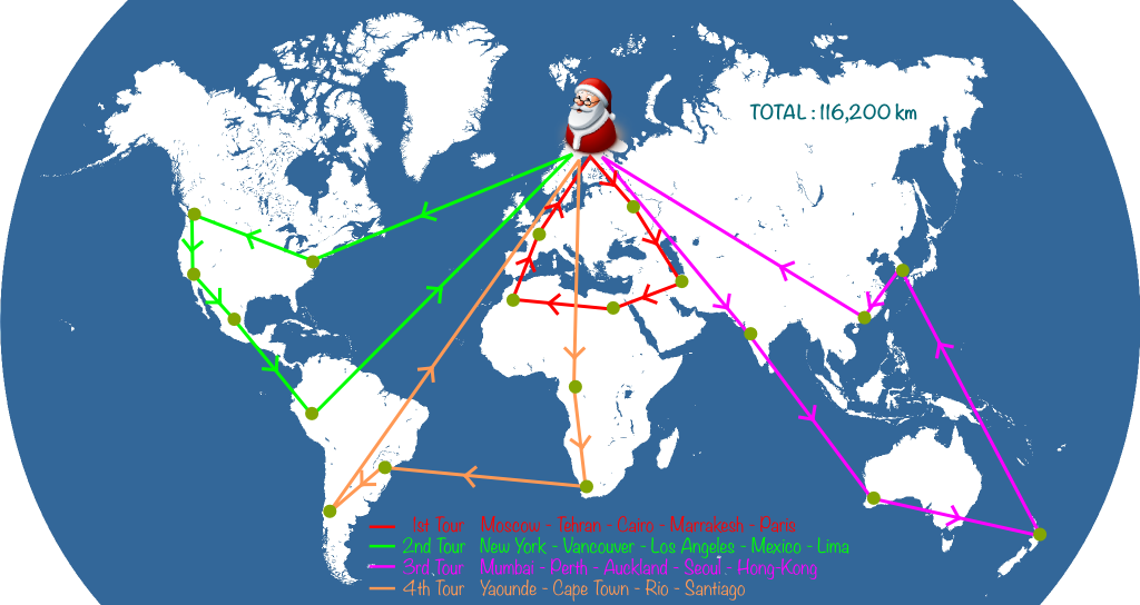
To make Santa Claus’ problem a vehicle routing problem, we merely have to assume that Santa Claus’ reindeers cannot carry too heavy quantities. So, for instance, they can only carry presents for 5 cities. This will force Santa to come back to his toy factory several times to reload his sleigh. Typically, a Santa’s journey on the night of December 24th could look as follows:

To have a chance to make it on time, it’s crucial for Santa to minimize the total distance of his journey. This corresponds to searching for a shortest overall journey. And that’s precisely what the Vehicle Routing Problem (VRP) is about.

The VRP is actually known to as hard as the TSP. This means that, when the number of cities isn’t small, there is virtually no hope to solve the VRP exactly in a reasonable amount of time, even with tomorrow’s greatest computer power. In fact, so far, no best solution is known for problems with more than a few hundreds of cities to visit!

So, rather than solving the VRP exactly, operational researchers have been designing clever technics to find nearly optimal solutions in a reasonable amount of time. These technics are called heuristics.

Greedy Algorithms

The most straightforward heuristics is the greedy algorithm.

It consists in choosing the next best step without much thinking, like a greedy Santa who is given a bunch of candies to choose from. He’d repeatedly eat his favorite one among the remaining candies, until he’s full… or until Mother Christmas tells him to stop!

It is! In many cases, like for Santa’s candies, the greedy algorithm turns out to be optimal!

A simple greedy algorithm would be to get Santa to the closest unvisited city.

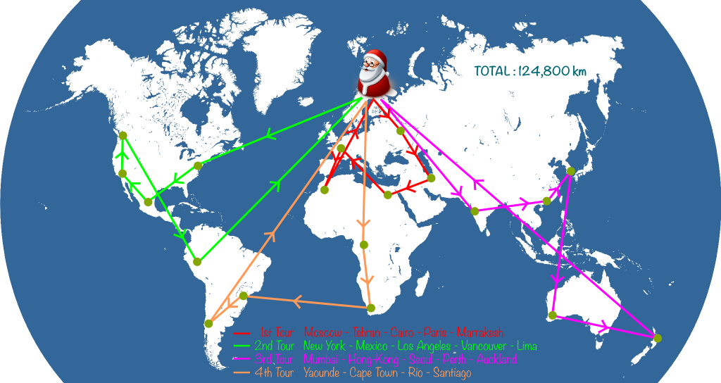
Sure! Starting in Santa’s workshop in Rovaniemi, and using this link, you can determine that the closest city is Moscow, at nearly 1,300 km. Then, the closest city to Moscow is Tehran. Then, the next closest cities to visit are Cairo, Paris and Marrakesh. Now that Santa has visited 5 cities, he must get back to Rovaniemi to pick up presents for other cities. Then, he goes on with his visits. Eventually, here’s the Santa’s journey we get:

Such a whole journey is called a solution. This is not to be confused with the optimal solution which would be the best Santa’s journey. Here, the solution found by the greedy algorithm is 124,800 kilometers long. Can we do better… And how?

Local Search

One way to do better is to improve what we have.

Hummm… Yes. But what I mean by that is that we can try to make small modifications to the best solution we’ve found, and see if these modifications lead to an improvement. This technic is called local search. It’s pretty much what people use when they play the colder-warmer game, where each step is warmer when it improves one’s location.

It’s up to you to invent them! Experiments characterized a simple and efficient kind of modification called 2-opt. It consists in removing two arcs and reconnecting cities of these arcs in a consistent way.

Sure! Let’s remove the arcs New York – Mexico and Vancouver – Lima. Then, we have two possible reconstructions. The New York – Lima and Vancouver – Mexico reconstruction breaks Santa’s tour so it’s not acceptable. Conversely, the New York – Vancouver and Mexico – Lima reconstruction is consistent with Santa’s tour:

Note that the paths we removed add up to 11,600 km, while these we’ve added in the consistent reconstruction add up to 8,200km. Thus, by modifying Santa’s 2nd tour, we’ve reduced the total distance by 3,400km!

Great observation! By removing 2 arcs that crossed in the 2-opt modification, I was sure to greatly improve the current solution! Let me apply that to all crossing arcs. This is what we get:

Network of Solutions

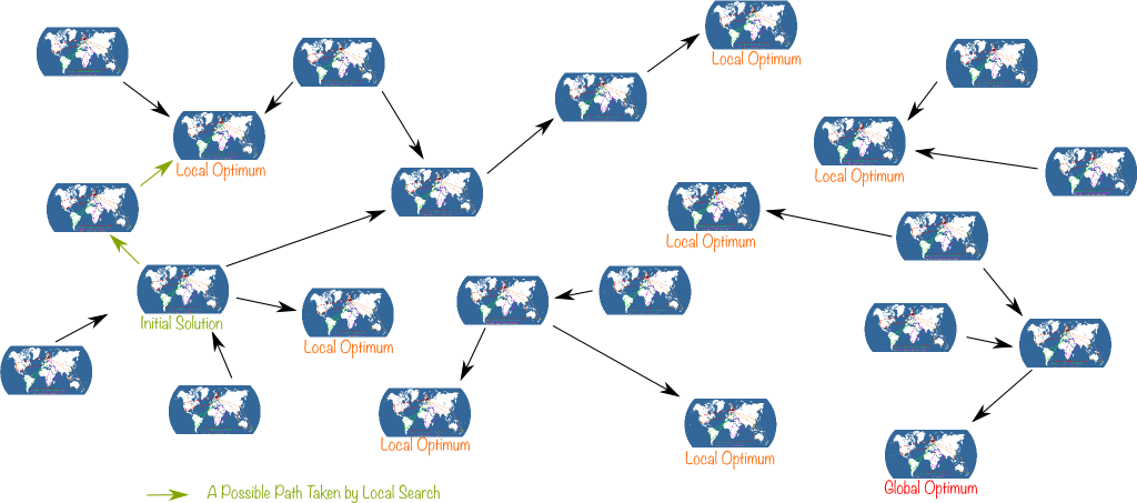
To fully understand what is meant by local search, let me introduce the network of solutions. This network connects two solutions if a 2-opt modification enables to move from one to the other. Typically, the following figure displays a few of the solutions of the larger network of solutions:

Any solution is connected to a bunch of others, which form what its neighborhood. And since we only looked at 2-opt modifications, our local search corresponds to exploring the neighborhood of best solutions found. So, the search is dubbed local, because we’re looking for better solutions only in the neighborhood of the current best solution.

In fact, let’s pause a bit on this network of solutions. Let’s forget about the details of the network and, rather, let’s ponder upon the global structure of the network of solutions…

Let’s look at the network as a cloud of solutions with connections between some of these solutions. When we apply a local search to this cloud, links can only be taken in certain direction: From the worse to the better solution. Thus, links actually have an orientation. In graph theoretical terms, this means that we actually have a directed (acyclic) graph of Santa’s journeys. And a local search will simply consist in taking a path in this graph until we face a dead-end.

I’d even add that it’s highly unlikely we will. One thing I can guarantee though is that we will reach a local optimum.

A local optimum is a solution which is better than any of its neighborhood. In other words, no arrow points out of a local optimum. So, crucially, it’s impossible with local search to get out of a local optimum. An that may be quite a problem, since a local optimum can be very bad compared to the global optimum.

Exactly! And there’s worse than the fact that our algorithm may not lead us to the global optimum: Depending on the initial solution, it may simply be impossible for local searches to get to the global optimum, as there may be no path from the initial solution to the global optimum! This remark has led to new ideas for optimization.

Adaptive Large Neighborhood Search

Building upon this remark, applied mathematicians have then invented the Adaptive Large Neighborhood Search (ALNS). The idea of ALNS is to make radical modifications of the current solution to move away from local optima. Sort of like you sometimes need a revolution to really change the world…

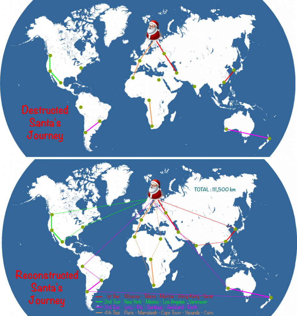
Typically, we’d only keep half of the arrows of the current solution, and try to fill the gaps using a basic method. It’s common to include randomness both in construction and destruction to make sure that we will rebuild a very different solution.

Sure. Let’s be clever and keep the arrows which seem relevant. Then let’s assign randomly colors to these arrows, and reconstruct afterwards how we can. Here’s what I got:

For good performance of ALNS, the level of destruction needs to be managed accordingly to the success of previous local search attempts. Note that there are several variants, like Variable Neighborhood Search (VNS) and Iterated Local Search (ILS).

Simulated Annealing and Tabu

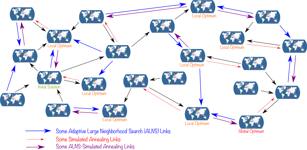
Indeed. This led to simulated annealing. The idea is to still carry out radical modifications even though they are worse than the current best solution, and as long as there is hope they will lead to good solutions after local searches. However, after more and more iterations, we may become more and more demanding and eventually require a strict improvement from the current best solution.

By analogy with metal annealing! In a hot metal, particles still jiggle around at all kinds of energy levels. Importantly, as long as the metal is hot, particles can leave low energy state and get to a higher energy one. But as the metal cools down, particles reach lower energy states and have more trouble leaving them. Eventually, they rest at a low energy state which is often lower than the one they’d reach had the metal been frozen instantly.

Exactly! Here’s how to visualize simulated annealing used combined to local search and ALNS:

Given the arrows of simulated annealing, a path may walk back on its footsteps. To avoid that, the Tabu search has been introduced. It simply consists in remembering the last footsteps made to makes sure we never come back to a solution we already explored.

Genetic Algorithms

In our example, combining all the heuristics discussed so far would yield nearly unbeatable solutions. But, as VRP models are made more realistic, they become much harder to solve, even heuristically! Examples of realistic constraints we may want to add include differences in quantity of toys required for cities, time windows to visit cities or reindeer required rests. For constraints like these, even slight modifications may greatly modify the quality of a solution. This leads to an explosion of the number of local optima. For this reason, the methods introduced so far can turn out quite limited.

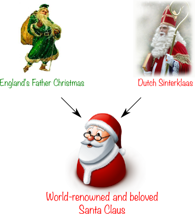
One great idea came from evolutionary biology: Genetic Algorithms. The core idea lies in the fact that a mixture of two parents can make a kid much better than the average of the parents. An example of that is how crossing English Father Christmas with Dutch Sinterklaas has given birth to the world-renowned Santa Claus.

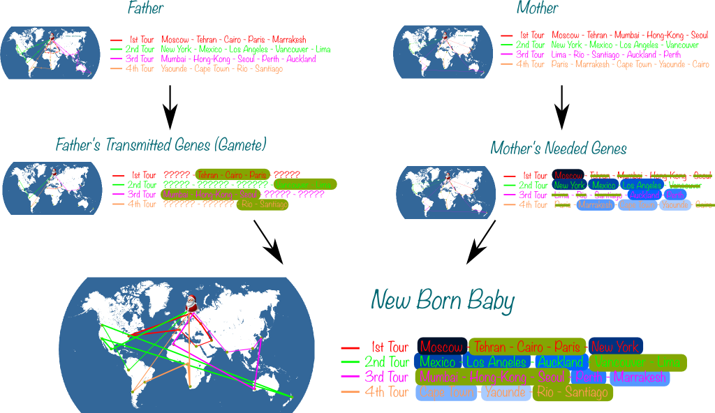
The key to powerful genetic algorithms lies in the way we cross the parents’ genes. Researchers have come up with plenty of ways to do so, as listed in this article. Let me consider one to illustrate.

First, we represent solutions as the ordered sequence of all visited cities. Then, the father solution yields half of the cities to the kid, all placed exactly as they appear in the father’s ordering of cities. The gaps are then filled by the other half of the cities, in the order in which they appear in the mother solution.

Sure. Let’s mix the greedy solution and the ALNS solution we have found earlier:

He needs education! Funnily, this term has been used to applying local search to the kid to make it an interesting solution!

But, at least, he’ll contribute to a greater diversity of solutions. Indeed, the problem with local search is that the intensification leads to solutions which all look the same. It’d be a bit like having all physicists working on string theory alone. Sure, string theory is promising and it probably deserves intensification… But if all physicists looked in a single direction, they’d be missing out on a lot of other less promising but eventually more fruitful leads! Conversely, many breakthroughs in History have resulted from a clever mix of good ideas, like how Newton merged Galileo’s laws of motions on Earth with Kepler’s laws of planetary motions!

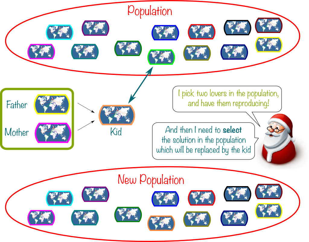
Exactly! A classical approach consists in maintaining a pool of diverse not-too-bad solutions, called population. This population can be initially generated by a greedy randomized adaptive search procedure (GRASP). Then, two solutions of the population are picked and crossed over. Their kid is inserted in the population and replaces an unfit or non-original solution of the population. The choice of the solution to remove is called selection, and it regulates the level of diversification. This is represented below:

Amazingly, since a paper by Christian Prins in 2004, genetic approaches have surpassed local searches in many problems.

Actually, genetic algorithms have been introduced as soon as the 1950s! But, crucially, computing power has greatly increased since, and you actually need to have this much greater computing capacity to get genetic algorithms running at their full potential!

I’m sure that their ideas will be useful. But I rather believe in even more advanced optimization technics.

Integer Programming and Cuts

Like most combinatorial optimization problem, the VRP can be written as an integer linear program.

It’s an optimization problems whose variables are all integers and which have a linear structure. More precisely, if you forget the fact that variables must take integer values, then you should be left with a linear program. This linear program has a linear objective function and linear constraints.

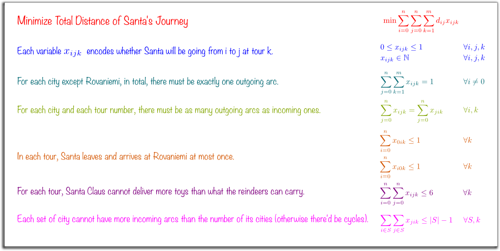
Let’s encode whether Santa goes from city $i$ to city $j$ in tour number $k$ by binary variables $x_{ijk}$. More, precisely $x_{ijk}$ equals 1 if Santa does, and 0 otherwise.

Now, to have an integer program, we also need an objective function and constraints.

It’s what we want to minimize (or maximize). So, in our case, it’s the total distance of Santa’s journey. Crucially, it can be deduced from the variables. Indeed, denoting $d_{ij}$ between cities $i$ and $j$, the term $d_{ij} x_{ijk}$ equals $d_{ij}$ if Santa goes from $i$ to $j$ in tour $k$, and 0 otherwise. Thus, by summing over all tours $k$ and over all pairs of cities $i$ and $j$, we add up all the distances of intercity trips of Santa: That’s also the total distance of Santa’s journey! So, VRP consists in finding the variables $x_{ijk}$ which minimize the sum of terms $d_{ij}x_{ijk}$ over all values of $i$, $j$ and $k$.

You’re right! And that’s because our integer program so far includes solution which are inconsistent with the actual VRP. We now need to add constraints to make the integer program consistent with the problem it’s supposed to solve.

Santa must go through all cities. In particular, if $i$ is a city which is not Santa’s, he must go through it exactly once. This implies that he must also leave it once. So, there must be one and only one variable $x_{ijk}$ which equals 1. Thus, all variables $x_{ijk}$ must add up to 1. So, for all cities $i$ different from Santa’s, we’ll add the constraint that the sum of $x_{ijk}$ equals 1.

Indeed. Let’s add the following constraints:

• Santa goes and leaves its home at most once in each tour (0 if he makes no visit in the tour).
• In each tour, through each city, there must be as many incoming arcs as outgoing ones.
• A tour cannot be made of more than 5 cities other than Santa’s (and thus 6 arcs).

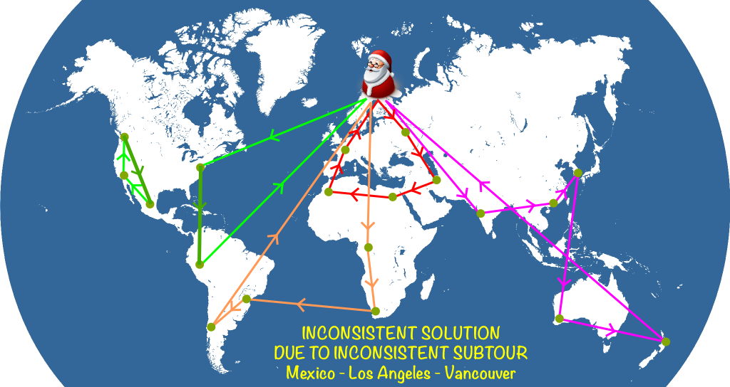
Now, given these constraints, it’s still possible to have inconsistent loops like below:

Such a solution is said to have a subtour. To avoid these, a common method is to add subtour elimination constraints. They are based on the two following remarks. First, for any subset $S$ of cities not including Santa’s, there must be at least one arc going out of the subset. Thus, this outgoing arc comes from a city which has no outgoing arc which remains in the subset $S$. Second, the number of arcs within the subset $S$ equals the number of cities of the subset with an outgoing arc remaining in the subset $S$. Thus, by combining the two remarks, we deduce that the number of arcs within $S$ cannot equal or exceed the number of cities of the subset!

Nope! We’re done! Here’s the complete integer programming formulation, with the mathematical translation of our constraints added on the right:

This formulation is nearly perfect to put it directly into an integer program optimizer and quickly get a great solution!

There’s one trouble though… The integer program above has an exponential number of constraints! Indeed, there are as many subtour elimination constraints as the number of subsets of the set of cities. And that’s bad, very bad…

If there are 100 cities, then there are $2^{100} \approx 10^{30}$ subtour elimination constraints! That’s more than the size of the web, which is only about $10^{18}$ bits! So, you can’t even write down the subtour elimination constraints for a VRP of 100 cities on the whole web!

Fortunately, applied mathematicians have more than a few tricks up their sleeves! They have proposed to start the optimization without subtour elimination constraints. Then, for each solution found, we add the subtour elimination constraints the solution does not verify. If there is no such subtour elimination constraint, then this means that our solution is consistent… And is the global optimum too! This technic is called cutting planes, and has turned out to be today’s state-of-the-art technique for many problems. In fact, other constraints than subtour eliminations can be used in cutting plane methods to efficiently reach quality solutions.

Let’s Conclude

So, would you now agree with Santa’s being a math genius?

Haha… Now, I should say that there’s one last more state-of-the-art optimization technic I have not mentioned here. And yet, it’s the specialty of my research lab! It’s called column generation, and exploits the structure of the integer program to write it differently, using the Dantzig-Wolfe decomposition. Find out more with this article!

Not at all. First, because other problems don’t have a structure as rich as the VRP does, which means that integer programming and column generation may not work for them, or would involve too much work and tests to get right. Second, and more importantly, these other methods can actually be used in combination with more advanced technics. This is particularly the case with column generation which decomposes the problem in smaller subproblems which may require local search or genetic algorithms! Overall, a clever balance of all these technics seems to be key for powerful optimization.

Yes! By now, there have been a huge number of variants of the VRP. Among others are VRPPD (where cities correspond to pick-up or deliveries, and capacities must be modeled accordingly), LIFO-VRPPD (where the order in which you load and unload goods in trucks matter), VRPTW (where each city must be visited within a certain time window), SDVRP (where deliveries for a customer can be split in several trucks), HVRP (where the fleet of vehicles is heterogeneous), SVRP and RVRP (with uncertainties where we minimize the average case or the worst case). And, these can be combined, yielding problems like LIFO-SDVRPPDTW… As you can imagine, I like to tease my VRP colleagues about how they create new problems by just adding letters to the acronym!