Many people believe that mathematics research is over. Yet, as I often retort to them, we still only know little of the immense ocean of mathematical structures, which, yet, fill the world we live in. One recent advancement is that of mean-field games around 2006, independently by Minyi Huang, Roland Malhamé and Peter Caines in Montreal, and by Jean-Michel Lasry and Fields medalist Pierre-Louis Lions in Paris. This revolutionary model has since been greatly developed by other mathematicians and largely applied to describe complex multi-agent dynamic systems, like Mexican waves, stock markets or fish schoolings.
Applications of mean-field games go way beyond the realm of animal swarms! Recently, Lasry and Lions exploited mean-field game theory to design new decision making processes for financial, technological and industrial innovation, as they launched the company mfg labs in Paris! Customers include banks and energy councils.
The Main Idea
Sometimes large numbers are much simpler than small ones. The core idea of mean field games is precisely to exploit the smoothing effect of large numbers. Indeed, while game theory struggles with systems of more than 2 individuals, mean-field games turn the problem around by restating game theory as an interaction of each individual with the mass of others.
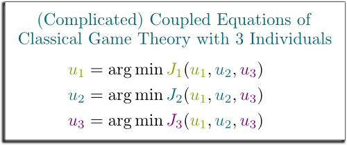
Imagine a fish in a schooling. In classical game theory, it reacts to what other fishes nearby do. And this is very complicated, as there is then a huge number of interactions between the different fishes. This means that classical game theory corresponds to a long list of highly coupled equations. Don’t worry if you don’t get what I mean. In essence, my point is that the classical game theory model becomes nearly impossible to solve with as little as 3 fishes, and it gets “exponentially harder” with more fishes.
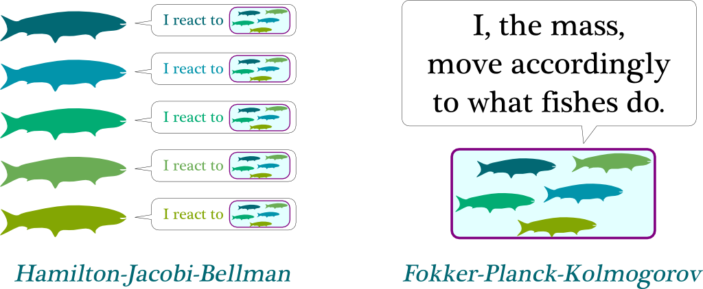
They are cleverly thought! In mean-field game theory, each fish does not care about each of the other fishes. Rather, it cares about how the fishes nearby, as a mass, globally move. In other words, each fish reacts only to the mass. And, amazingly, this mass can be nicely described using the powerful usual tools of statistical mechanics!
Granted, the motion of the mass is necessarily the result of what each fish does. This means that we actually still have coupled equations, between each fish and the mass.
On one hand, the reaction of fishes to the mass is described to the Hamilton-Jacobi-Bellman equation. On the other hand, the aggregation of the actions of the fishes which determines the motion of the mass corresponds to the Fokker-Planck-Kolmogorov equation. Mean-field game theory is the combination of these two equations.
Don’t worry, it sounds way more complicated than it really is! Bear with me!
Hamilton-Jacobi-Bellman
Before getting further, I need to have you pondering upon a simple question… What can fishes do?
I’m not sure Newton would have liked this answer… Isn’t it rather acceleration that’s in their control?
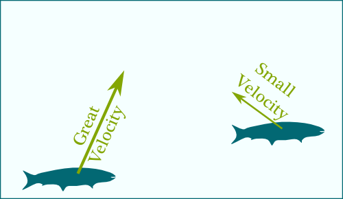
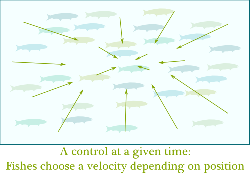
Humm… This is getting complicated. So, let’s assume that, as you first said, fishes can move however they want. Mathematically, this means that they control their velocity, which is an arrow which points towards their direction of motion. Plus, the longer the arrow the faster fishes swim. So, at any time, a fish controls its velocity, depending on where it is, and where the mass is.
I’m going to define one of the two main objects of mean-field games: the control $u$. A control is a choice of velocity depending on position and time. Crucially, if all fishes are similar, then they all have the same optimal control. Thus, we only need one control $u$ to describe the actions of all the fishes!
Hummm… The concept of what’s a best control for fishes is quite debatable. But, for simplicity, let’s say that a good control should get fishes close to the schooling where it is safer, while avoiding abusing great velocities which are fuel-consuming.
Crucially, a good control doesn’t only care about what’s best for the fish right now. It must also consider where the fish should go for it to be safe in the future.
Basically, at each point of time, a fish pays the unsafeness of its position and the exhaustion due to its velocity. Its total loss over all time simply consists in adding up all the losses at all times. Thus, the fish must strike a happy balance between hurrying to reach a future safer position and not running out of energy at present time. This setting is known as an optimal control problem.
Optimal control is solved like chess! In essence, we should first think of where we should get to, and then work backwards to determine which steps will get us there. This is what’s known as dynamic programming.
I totally agree with you. But I don’t name stuffs!
First, we start by judging how costly the possible future positions are. This gives us a map of total future costs. Now, ideally, no matter where a fish is, he’d prefer to get to the least costly future position. However, there’s also a cost due to motion:
Now, given a present position, we’ll want to choose a velocity which minimizes the sum of future total costs and velocity cost.
Sure! Look at the figure below. On the left, the present position is assumed to be where arrows go out from. Staying still has a future total cost of 4, and no velocity cost. Meanwhile, moving one step to the left yields a future total cost of 2 and a velocity cost of 2, which add up to 4. What’s more, moving one step below adds a future total cost of 1 and a velocity cost of 2, adding up to 3. Thus, moving below is less costly than moving to the left or staying still. In fact, it’s the least costly move. This is why the optimal control consists in moving downwards. Interestingly, now that we know what the optimal control at the present position is, we can derive the present total cost, which is the sum of present unsafeness (1), future total cost (1) and velocity cost (2): 4.
Now, by doing so for all present positions, we can derive the full optimal control at present time, as well as the map of present total costs!
Excellent remark! Well, by increasing the details of discretization, and following Newton’s steps, we can in fact derive a continuous version of dynamic programming. This yields the famous Hamilton-Jacobi-Bellman equation, which, in essence, is simply the continuous extension of dynamic programming!
Fokker-Planck-Kolmogorov
So, if I recapitulate, the Hamilton-Jacobi-Bellman tells us how fishes react to the mass. But, as we’ve already discussed it, the mass is derived from what the fishes do.
Excellent question! The mass $m$ describes all trajectories of all fishes.
There’s a way to make it sound (slightly) less frightening: Let’s imagine all the possible trajectories. Then, we can simply have $m(x,t)$ counting the ratio of fishes which happen to be at position $x$ at time $t$.
Now, as opposed to the backward Hamilton-Jacobi-Bellman equation, we are now going to work forward: We’ll derive the mass of the near future, from the present mass and the control.
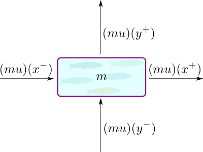
We first need to notice that the velocities given by the control aren’t very relevant to describe how the mass moves. Instead, as noticed by statistical mechanics, what rather matters is the “quantity of motion” of fishes, which physicists call momentum. This momentum really is what describes how fishes move. At a given point, this momentum corresponds to the velocity multiplied by the number of fishes in motion. It is thus the vector field $m(x,t) \cdot u(x,t) = (mu) (x,t)$. Now, by adding up all the quantities going in and out of a point we obtain the Liouville equation.
But the Liouville equation features no Brownian motion.
Yes, I need to explain that! The thing is that, if fishes follow the Liouville equation, they’ll all end up converging to the single safest point. That’s not what happens in reality. While fishes would probably like to all be in the middle of the schooling, there may not get a chance, as the crowdedness will have them knocking one another. One way of interpreting that, is to say that they won’t be in total control of their trajectories, kind of like a grain of pollen floating in water.
In fact, this motion of the grains of pollen was discovered by botanist Robert Brown in 1827, and it is what we now call the Brownian motion. This Brownian motion has played a key role in the History of science, as it was what led Albert Einstein to prove the existence of atoms! This is what I explained it in my talk More Hiking in Modern Math World:
For our purpose, the important effect of Brownian motion is that there is a natural tendency for fishes to go from crowded regions to less crowded ones. Thus, while safeness makes fishes converge to a single safest point, the Brownian motion spreads them in space. The addition of the latter idea to the Liouville equation yields by the famous Fokker-Planck equation, also known as the Kolmogorov forward equation, and which I’ll name the Fokker-Planck-Kolmogorov equation here.
Time-Independency
One natural setting in which to study mean-field games is that where there is a perfect symmetry in time. This means that the costs $g$ don’t depend in time and that there is no end time.
I know, it sounds weird. After all, fishes eventually die, so there has to be an end time. But if this end time is so far away compared to the reaction time scales of the fishes, and it’s the case in practice, then it’s very natural to approximate the very large end time by infinity.
Crucially, now, the controls $u$ no longer depend on the time variable. They are just instructions that give a velocity to be taken depending on position. This means that, at each point of space, there is a velocity to take. This is what physicists call a vector field.
Absolutely! The mass is now merely described by an unchanging variable $m$. This means that the mass of fishes is remaining still. Or, rather, since this is up to switch of inertial system, that fishes are moving altogether at the same velocity (up to Brownian motion, and along the current to minimize kinetic energy).
Hehe… That’s an awesome question. Well, we’d need to get back to the time-dependent case, and include some perturbations of the map of unsafeness, which may be due, for instance, to the apparition of a predator! I’ve never seen simulations of that, but I trust the maths to make it awesome!
Linear-Quadratic Games
In this article, whenever I gave formulas so far, I assumed we were in a (nearly) linear-quadratic setting. This means that the control linearly determine the velocity (like in the formula $u=\dot x$, or more generally, if $u=a\dot x + b$`), that the cost of velocity is quadratic (as in the kinetic energy $^1/_2 ||u||^2$), and that the unsafeness of position is also quadratic (which, in fact, we don’t need to state the theorems of this last section). Crucially, this makes the Hamilton-Jacobi-Bellman equation easy to transform into a partial differential equation.
Not only do these assumptions enable us to write nice-looking partial differential equations, they also imply three holy results mathematicians are always searching for.
The two first ones are very classical. Yes, you know what I’m talking about: existence and uniqueness.
Because, if we want our equations to have a chance to describe reality, then their solutions must share one important feature with reality. Namely, they must exist, and they must be unique. More generally, especially in the field of partial differential equations, existence and uniqueness of solutions often represent the Saint-Graal, or, at least, an important mathematical question.
Sure, people do! But since these equations usually can’t be solved analytically, we usually turn towards numerical simulations. These simulations typically discretize space and time and approximate the equations. However, while these numerical simulations will run and engineers may then make decisions based on their outcomes, if the equations didn’t have a solution to start with, or if they had several of them, then the results of the simulations would then be meaningless! Proving existence and uniqueness yields evidence for the relevancy of numerical simulations.
In fact, one of the 7 Millenium Prize problem, called the Navier-Stokes existence and smoothness problem, is precisely about determining the existence and uniqueness of solutions to a partial differential equation, as I explain it later in my talk More Hiking in Modern Math World:
In the linear-quadratic setting with Brownian motion, they do! How cool is that?
The third result is that the solutions can be computed! While classical partial differential equations are solvable by numerical methods, mean-field game equations are a bit trickier as they form coupled partial differential equations. More precisely, given the mass $m$, we can compute the optimal control $u$ with the Hamilton-Jacobi-Bellman equation; and given the control $u$, we can derive the mass $m$ from the Fokker-Planck-Kolmogorov equation. But, at the beginning, we don’t know any of the two variables!
Through an iterative process! Let’s start with an arbitrary mass $m_0$.
Then, we’ll compute the corresponding optimal control $u_1$, from which we then derive the mass $m_1$. And we repeat this process to determine $u_2$ and $m_2$, then $u_3$ and $m_3$… and so on. Crucially, this iterative process will yield the right result, as, in some sense I won’t develop here, the sequence $(u_n, m_n)$ converges exponentially quickly to the unique solution $(u,m)$ of the mean-field game couple partial differential equations!
Let’s Conclude
It’s interesting to note that the Hamilton-Jacobi-Bellman equation comes from control theory (which is often studied in electrical and engineering departments), while the Fokker-Planck-Kolmogorov equation first appeared in statistical mechanics. And yet, it is in game theory that their combination has yielded the most relevant models! The story of the creation of mean-field game theory really is that of the power of interdisciplinarity in innovation processes! And yet, I’m confident in the fact that the full potential of mean-field games has not yet been found, and that some hidden mind-blowing applications are still to come!
Exactly! As weird as it sounds to many, mathematics is more than ever a living and dynamic field of research, with frequent discoveries and conceptual breakthroughs! Which leads me to advertise my own ongoing research… The first part of my PhD research is actually a generalization of mean-field games. Crucially, the key step of mean-field games occurred early in this article, as we restated classical game theory in terms of other interacting variables: The control $u$ and the mass $m$. More generally, in game theory, we can similarly decompose games into two interacting components: The strategies played by players, and the so-called return functions, which I got to name since it’s my very own creation!
Hehe! Stay tuned (by subscribing)… as I’ll reveal everything about these return functions once my (recently submitted) research paper gets published!




Thanks, the article is really helpful and the main idea of mean field games is very well-explained.
Hello Sir,
Excellent explanation, i was looking for some material on Mean field games, and i found this, once again, very neat and clean way of explanation. Its hard now a days to find some literature like this, you put way hard effort in this. Once again, the best article on mean field games.
Do share the links of your other articles in the field of game theory, or if you have a personal blog or website then please share a link. I want to explore more.
Thanks a lot !
Regards,
A Student