Duality is a concept from mathematical programming. In the case of linear programming, duality yields many more amazing results.
The dual linear program
The duality theory in linear programming yields plenty of extraordinary results, because of the specific structure of linear programs. In order to explain duality to you, I’ll use the example of the smart robber I used in the article on linear programming. Basically, the smart robber wants to steal as much gold and dollar bills as he can. He is limited by the volume of his backpack and the maximal weight he can carry. Now, let’s notice that we can write the problem as follows.
$$\textrm{Maximise} \quad \textrm{Value}_\textrm{gold} volume_\textrm{gold} + \textrm{Value}_\textrm{bills} volume_{\textrm{bills}} \\\\
\textrm{Subject to} \quad volume_{\textrm{gold}} + volume_{\textrm{bills}} \leq \textrm{Volume}_{\textrm{limit}} \\
\textrm{} \qquad \qquad \quad \;\; \textrm{Density}_\textrm{gold} volume_{\textrm{gold}} + \textrm{Density}_\textrm{bills} volume_{\textrm{bills}} \leq \textrm{Weight}_{\textrm{limit}} \\
\textrm{} \qquad \qquad \quad \;\; volume_{\textrm{gold}} \geq 0 \\
\textrm{} \qquad \qquad \quad \;\; volume_{\textrm{bills}} \geq 0$$
The problem we have written here (no matter which equivalent formulation we used) is what we call the primal linear program. It’s now time for you to learn about the dual linear program! The dual program will totally change our understanding of the problem, and that’s why it’s so cool. I hope you are as excited as I am!
In the primal program, constraints had constant numbers on their right. These constant numbers are our ressources. They say what we are able to do concerning each constraint. The dual problem consists in evaluating how much our combined ressources are worth. If the offer meets the demand, our ressources will be just as much as their potentials, which is the worth of the robbery. Sweet, right?
Let’s go more into details. In the dual problem we will attribute values to the ressources (as in “how much they’re worth”). These values are called the dual variables. In our case, we have two constraints, so we will have 2 dual variables. The first dual variable, let’s call it $value_{\textrm{volume}}$ refers to the value of one unit of volume. As you have figured it out, the second dual variable refers to the value of one unit of weight. $value_{\textrm{weight}}$ seems like a right name for it, right?
Now, I bet you can write the value of the robbery with these two new variables… Let’s see if we get the same result.
$$\textrm{Total Value} = value_{\textrm{volume}} \textrm{Volume}_{\textrm{limit}} + value_{\textrm{weight}} \textrm{Weight}_{\textrm{limit}}$$
If I wanted to sell my ressources, potential buyers are going to minimize the value of my ressources. So their valuations are the minimum of the total value. But as a seller, I will argue that each of my ressource is worth a lot, because it enables the robbery of more gold and more bills.
Obviously, the values of ressources depend on the actual values of gold and bills per volume. Let’s have a thought about the value of gold (and then you’ll be able to apply the same reasoning to bills). If the constraints enabled us to steal one more volume of gold, then incremental value of the robbery would be at least the value of this one volume of gold, right? It could be more, if we use the new constraints to steal something else than gold that’s worth more. What I’m saying is that, if the total volume enabled us to steal one more unit of volume of gold, and if we could carry one more unit of weight of one volume of gold, then the value of this incremental steal would be at least the value of one more volume of gold. Let’s write it.
$$value_{\textrm{volume}} + value_\textrm{weight} \textrm{Density}_\textrm{gold} \geq \textrm{Value}_\textrm{gold}$$
I’ll let you write the similar constraint for bills. In fact, we can do this reasoning with any variable of the primal problem and ask ourselves the question: “If we add one unit of the variable, how will it affect the total valuation?” From that we deduce a constraint on dual variables. As you see, any variable in the primal problem is associated with a constraint in the dual problem and vice-versa.
We are almost done. Let’s notice the fact that if we increase the total volume, then we have more possibilities for the primal variables, which are the volumes of stolen gold and bills. Therefore, the value of a unit of volume cannot be negative. This adds two more constraints on the sign of dual variables. Now, we’re done and we can write the dual problem.
$$\textrm{Minimise} \quad value_{\textrm{volume}} \textrm{Volume}_{\textrm{limit}} + value_{\textrm{weight}} \textrm{Weight}_{\textrm{limit}} \\\\
\textrm{Subject to} \quad value_{\textrm{volume}} + value_\textrm{weight} \textrm{Density}_\textrm{gold} \geq \textrm{Value}_\textrm{gold} \\
\textrm{} \qquad \qquad \quad \;\; value_{\textrm{volume}} + value_\textrm{weight} \textrm{Density}_\textrm{bills} \geq \textrm{Value}_\textrm{bills} \\
\textrm{} \qquad \qquad \quad \;\; value_\textrm{volume} \geq 0 \\
\textrm{} \qquad \qquad \quad \;\; value_\textrm{weight} \geq 0 $$
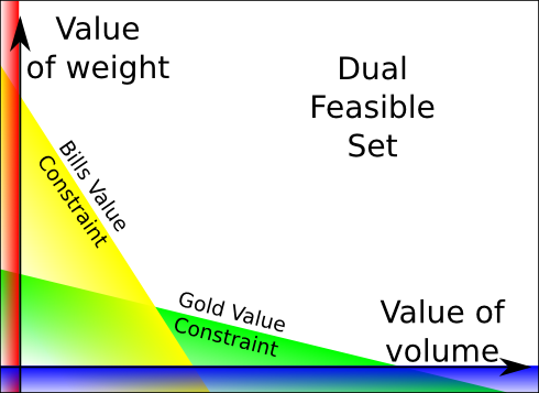
And it always does! The dual program of a linear program is a linear program! Let’s have a look at the feasible set.
It’s important to notice that the information of the primal objective functions appear in the dual feasible set. However, it loses the information of the primal ressources. This information would appear if we draw the level sets of the dual objective function. Nevertheless, if we draw the primal and dual feasible sets, then we have all the information of the linear programs.
The most important result is the strong duality property: optimal values of the primal and dual problems are the same. We can solve the primal problem simply by solving the dual problem! And sometimes, the dual problem can be much more simple than the primal one.
What’s more, and that’s less obvious here, the dual of the dual is the primal. This can be proved with calculus. Try to transform the dual program into a maximisation program with less or equal inequality constraints to find its dual, that’s a good exercise. But what’s interesting is the real reason why the dual of the dual is the primal. Try to think about it. It’s very tricky but even more interesting exercise. This means that the value of the ressources of the dual constraints are the primal variables. In our example, if the value of gold increases by 1 unit, then the worth of the robbery would be increased by the quantity of stolen gold. This means that the value of the value of gold is the quantity of stolen gold!
There’s something else quite interesting about duality: It gives directly a sensitivity analysis. Consider our primal problems. It’d be interesting to know how much more I could get, had my knapsack been larger or my body stronger. This looks like a difficult question in the primal program, but it’s very obvious in the dual program. If I can have one unit of volume more in the knapsack, then the incremental worth of the robbery will be $value_\textrm{volume}$. This is actually a minimizer of the incremental worth I’ll have, but it’s a perfect approximation for small incremental volume of the knapsack.
But that’s not all. In linear programming, duality yields plenty more of amazing results! In particular, there is a strong connection between the primal bases and the dual bases.
Dual bases
Let’s notice that the primal problem is equivalent to the following formulation.
$$\textrm{Maximise} \quad \textrm{Value}_\textrm{gold} volume_\textrm{gold} + \textrm{Value}_\textrm{bills} volume_{\textrm{bills}} \\\\
\textrm{Subject to} \quad volume_{\textrm{gold}} + volume_{\textrm{bills}} + volume_{\textrm{unused}} = Volume_{\textrm{limit}} \\
\textrm{} \qquad \quad \;\; \textrm{Density}_\textrm{gold} volume_{\textrm{gold}} + \textrm{Density}_\textrm{bills} volume_{\textrm{bills}} + weight_{\textrm{unused}} = Weight_{\textrm{limit}} \\
\textrm{} \qquad \qquad \quad \;\; volume_{\textrm{gold}} \geq 0 \\
\textrm{} \qquad \qquad \quad \;\; volume_{\textrm{bills}} \geq 0 \\
\textrm{} \qquad \qquad \quad \;\; volume_{\textrm{unused}} \geq 0 \\
\textrm{} \qquad \qquad \quad \;\; weight_{\textrm{unused}} \geq 0. $$
This equivalent formulation has introduced the two variables $volume_{\textrm{unused}}$ and $weight_{\textrm{unused}}$. These variables are called slack variables. Any linear problem can be written with slack variables and a full rank matrix $A$ to have the following form.
$$\underset{x,e}{\textrm{Maximise}} \quad c^Tx \\
\textrm{Subject to} \quad Ax + e = b \\
\textrm{} \qquad \qquad \quad \;\; x, e \geq 0.$$
We can obtain a similar formulation for the dual program.
$$\underset{y,s}{\textrm{Minimise}} \quad y^Tb \\
\textrm{Subject to} \quad y^TA – s^T = c^T \\
\textrm{} \qquad \qquad \quad \;\; y, s \geq 0.$$
Don’t worry, it’s not that important. It’s not even a standard formulation. I like this formulation because it shows the similarity between the primal and dual programs. It’s also a nice way to describe duality and its properties. Be careful with other formulations. The results I’ll give here can be hard to translate to other formulations.
What you need to notice is that we now have variables represented by vectors $x$, $e$, $y$ and $s$. Also, each variable of the vectors $e$ and $s$ appears alone in one of the constraints of the primal or dual program.
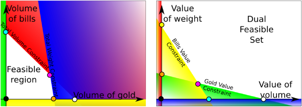
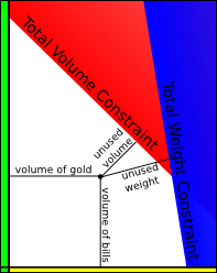
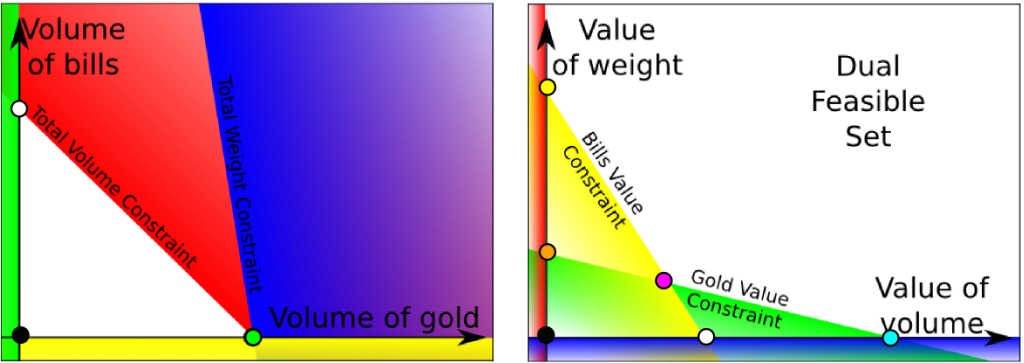
The variables can easily be understood in the following graph. The initial variables $x$ are the coordinates of the points, while the slack variables represent the distances from the different constraints. The unit of the slack variables is a little bit more complicated. To imagine it, keep in mind that the limits of the constraints are level sets. These level sets move as the value of they take varies.
Let’s denote $n$ the number of variables of $x$, and $m$ the number of variables of $e$. Note that $n$ is the number of constraints in the dual program, and $m$ is the number of constraints in the primal program. Therefore, a primal base is defined by the choice of $m$ variables which values will be set to zero. These $m$ variables form the “constraint base” I mentioned in the article on linear programming. The $n$ other variables are the “base”, in the usual definition of it.
What’s interesting is that the dual bases behave in the opposite way. As a matter of fact, they require $n$ variables in the constraint base and $m$ variables in the base. What’s even more interesting is that we can match each primal base to a dual base. As a matter fact, each variable of the vector $y$ corresponds to a constraint, which corresponds to a variable of the vector $e$. Similarly, we match variables of vectors $x$ and $s$. Therefore, to any primal base we can associate a dual base by choosing to add in the dual base variables that match the primal variables that are not in the primal base. Another way of saying it is that whenever we have not fixed a primal variable to 0, we fix the corresponding dual variable to 0.
This gives us the following matching of bases (drawn by the colors of dots).
The constraints of the two graphs can be matched. Non-negativity constraints of initial variables correspond to actual constraints in the other other program. A base defined by the intersection of two colors of constraints in one problem is matched with a base defined by the intersection of the two other colors of constraints in the other problem. On the two graphs, only the primal base associated with the dual yellow base has not been drawn, because the primal intersection of green and blue constraints could not be drawn.
Wait… There’s even more interesting: the values of the objective function of a primal base and its associated dual base are the same! Considering the way we introduced the dual program, this is very surprising. You may prove it with calculus, but the real reason why we have such a result involves the construction of the Lagrangian. If we had done that, we could have easily proved that, for any primal and dual variables satisfying the equality constraints, the difference of the primal by the dual objective functions is equal to $s^Tx + y^Te$. This value is called the complementary slackness. It is nil if the dual variables correspond to the dual base of the primal variables.
As a matter of fact the two programs have the same values. Since the primal program is a maximization problem, the value of its objective function is always less than the optimal value. And it’s the opposite for the dual program. Yet, this reasoning works for variables in the feasible set only! Therefore, the optimization problem is equivalent to finding a primal feasible base with an associated dual feasible base!
On the two graphs, only the pink dots are primal and dual feasible: they represent the solution of the linear programs!
Yes we can. And this gives us… the simplex method! As a matter of fact, the simplex method consists in moving from primal feasible base to strictly better primal feasible base. But it can be equivalently considered as an algorithm that moves from primal feasible bases to primal feasible bases with an associated dual base that gets more and more feasible. This “close-to-feasibility” criterium can, for instance, mean having the most negative variable as close to 0 as possible. Once the most negative variable of the dual base is non-negative, we have a dual feasible base. Therefore, we have reached the optimum.
Similarly, we could move from feasible dual bases to feasible dual bases, as we try to reach an associated feasible primal base. This is equivalent to applying the simplex method to the dual program and is known as the dual simplex.
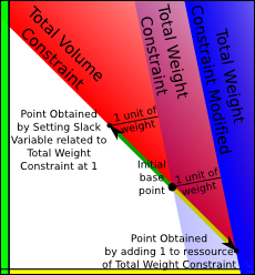
As you can imagine with this remark, there is a huge link between dual variables and reduced costs. This can be observed in the graph on the left. A reduced cost tells you by how much the objective function will increase if you lose one of the constraint of the base constraint and walks away from it on the edge defined by the other constraints of the constraint base, by 1 unit of the slack variable associated with this constraint. This reduced cost is the incremental value of the objective function when moving along the green arrow.
That’s almost the same thing as the dual variables that will tell you by how much the objective function will increase if you move one of the constraint by 1 unit of the ressource. This is the incremental value of the objective function when moving along the yellow arrow.
As you can see on the graph, the dual variable is the opposite of the reduced cost of the slack variable associated to the dual variable. Be careful with the sign. Our result is valid here because we have less or equal inequalities in the primal program (or, equivalently, the slack variables are preceded by a “+”). If we had higher or equal inequalities or slack variables preceded by a minus, we would have the equality of the reduced costs and dual variables.
That’s an awesome idea! It leads to… the interior point method! The idea of the interior point method is to remain inside the feasible set and to converge towards the optimum. This avoids the possibly numerous iterations to go from extreme points to extreme points, and it skips problems of degeneracy. For great numbers of variables, the interior point method is faster than the simplex method.
Given a positive real number µ, the interior point method consists in finding the primal and dual vectors that satisfy the equality constraints, are positives, and such that the product of each primal variable with its associated dual variable is equaly to µ. Then, as we decrease the value of µ, we approach to the primal and dual optimal solutions. The advantage of such a method is that we can use gradient-based algorithms to optimize the problem, which guarantee a very quick resolution. Another very interesting advantage is that it can be generalized to semi-definite programming.
As you see the dual program yields plenty of extraordinary results and provides a very interesting different understanding of the problem. Unfortunately, it faces the problem of degeneracy, especially when applying the simplex method.
Degeneracy
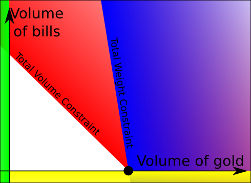
In our example, each primal base or constraint base matches one unique point. Yet, it’s possible that three constraints intersect at the same point, in which case, any combination of two of these three constraints correspond to that point. The matching is no longer unique. This situation happens for instance in the following case at the black dot.
It’s bad for the simplex algorithm. First it forces us to make a choice. Suppose that we were at the constraint base defined by the green and yellow constraints, and that the simplex algorithm decides to lose the green constraint. Then, we would move along the yellow constraint until we reach the black dot. This black dot can be defined by the fact that we’ve intersected the red or the blue constraint. One of them will be added to the constraint base. We need to make a choice. This is actually not really a problem. But the remark is a big problem.
Suppose the blue and yellow constraints form the constraint base (which means that slack variables corresponding to green and red constraints are in the base). If we put the yellow constraints out of the constraint base, then we would move along the blue line away from the yellow constraints. The direction along the blue constraint improves the objective function, which means that it’s associated with a positive reduced cost. Therefore, we should expect a strict increase of the objective function. Yet, because of the red constraint intersecting at the black dot, the red constraint would be added to the constraint base, which therefore will define the same black dot. We have made an iteration of the simplex method without improving anything.
If we handle the situation badly, it’s possible in certain cases to never get out of the black dot. Theoretically, we could apply the Bland’s rule to avoid that from happening. However, even with this rule, the resolution could be extremely long for very degenerated points (I mean points that can be defined by a lot of different bases). Imagine the case where the dimension of the feasible set is 25 and where we have 50 constraints intersecting at the same point. Then the number of bases defining this point is $\binom{50}{25} \approx 10^{14}$. The Bland’s rule has a good chance to visit half of them… This would take like forever! Maybe days… That’s very very bad. And yet, a dimension of 25 is very small.
We could thought of adding slight disturbances on constraints. This would avoid degeneracy. However, it wouldn’t really improved the resolution, as it would create multiple points very close to each other. The simplex method would still move around these points with very small improvement of the objective function. Basically, there is still a good chance of visiting half of all the bases associated to the degenerated point, so that’s still not good. Such cases are so similar to degeneracy that they can be considered as such.
The problem of degeneracy is often dealt by managing the set of constraints and the set of variables. In our case, if we could detect that the primal blue constraint was useless, then we would have solved the problem of degeneracy. In Montreal, several methods like the Dynamic Constraint Aggregation (DCA), the Integral Primal Simplex (IPS) and the Improved Column Generation (ICG) have also been developed. Briefly said, I’d say that they classify variables depending on how they appear in the constraints and solve over a small group of variables only. They may look into other variables if the optimality criterium is not satisfied. Find out more with my article on column generation.
Now, the reason why I have decided to talk about degeneracy in an article on duality is because duality offers an interesting understanding of degeneracy.
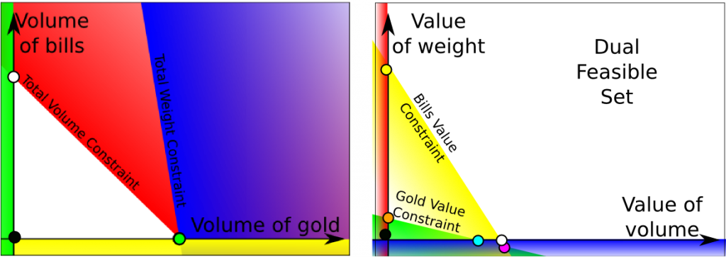
Let’s notice that the dual feasible has not changed if we only modified the ressource of the weight constraint. Therefore we have the following matching.
As you can see on the graph, there are fewer base points in the primal than in the dual. In fact, the primal green dot can be matched with the dual cyan, pink and orange dots. In fact, the primal green extreme point is actually associated with the dual green constraint.
No. Let’s denote n the dimension of the primal feasible set. Consider a degenerated point. Let’s call degeneracy is the number of constraints that are not required to define it. Let’s denote d the degeneracy. In our case, the degeneracy d is equal to 1. Then the number of non-nil primal variables at this point is equal to n-d. Therefore, the number of dual constraints that are in all the dual constraint bases associated to the degenerated point is n-d too. Their intersection defines the dual space associated to the degenerated point. As the dual space requires n constraints to define a point, the dual space associated to the degenerated point represents a vector space of dimension d. It matches a constraint if d = n-1, but is usually a vector space with a smaller dimension. As this whole vector space matches a single primal point that has a single objective value, the whole vector space has a single objective value. Therefore, the whole vector space is included in a dual objective function level set.
In the example, there are several primal-dual feasible bases, defined by the matching of the primal green and dual pink dots, and by the matching of the primal green and dual white dots. Degeneracy at the optimum is actually equivalent to the existence of several primal-dual solutions. From that, we can deduce that the dual cyan, pink and orange dots have a same dual objective value, which means that the green constraint is a level set of the dual objective function.
Let’s make our degenerated point non-optimal to see what happens. In order to do that, we’ll assume that the value of gold has suddenly dropped, making the primal white dot optimal. As a result in the dual the green constraint will be lower (look at its definition if you want to make it sure). We obtain the following graph.
The green constraint still represents the dual set associated with the degenerated point. However, in this case, this whole dual set is infeasible.
What’s interesting to notice is that it’s not possible to go directly from the dual orange dot to the dual optimal white dot. In the primal problem, this means that if the constraint base contains the blue and yellow constraints, it will not be able to go directly to the primal optimal white dot. More generally, there may be plenty of dual bases associated to a degenerated point that do not enable leaving the degenerated point. In a dual viewpoint, this means that we have to move all along a dual infeasible polyhedron without improving the dual objective function. Once at a degenerated point, it is therefore crucial to find a right associated dual point that will give us a way to get out of the degenerated point.
The Dual Variable Stabilization (DVS) follows this idea. It was proved to be efficient to deal with such cases, especially in the case of column generation. The idea of it is that once iterations of the simplex give close dual points, we add a penalty to dual points far from those we have recently found. Read my article on DVS to better understand it.
Let’s sum up
Duality yields plenty of amazing results. In particular, one very interesting thing to do is to observe what happens in the dual when we apply the simplex method or the interior point method to the primal linear program. For the simplex method, this naturally defines a new method called the dual simplex method. Learn more by reading my article on simplex methods.
An important application of the duality theory is the definition of the prices of the ressources. This is the case in the Location Marginal Price (LMP) algorithm used in electricity markets. As a matter of fact, this algorithm consists in minimizing the total cost of production of electricity with constraints on the demand at each geographical location. The demand can be viewed as ressource. If the demand at a location increases, then it would cause an incremented cost of production of electricity. In the electricity market, this incremented cost is considered as the price of electricity at that point. It’s a great model that takes into account electricity losses for instance. If a demand is at a location far from generators that induce plenty of losses, an increase of the demand at that location will induce an important incremental production, hence a higher incremental cost of production. Therefore, the dual variable associated to the demand, which is the price, will be higher.




That is a well thought out explanation. Now I have a profound understanding of what Dual does. Thank you very much.