Statistician Valen Johnson recently published an earth-shaking proceeding which asserts that 17 to 25% of published scientific results may simply be wrong.
Johnson explains this by a mere statistical consequence of the 5% rule. Fortunately, this accounts for wrong results without requiring any non-ethical behavior of experimentalists!
Basically, scientists are asked to make sure that no more than 5% of their results indeed false positive. Yet, because most published results are the most impressive ones (which include most false positives), Johnson claims that this has led experimentalists with up to a quarter of false positives among all published positives!
I agree! Johnson proposes to lower the standard (but greatly arbitrary) bound of 5% to 0.5%, or even to 0.1%.
Oh yes. Let me show you how this works, as I’ll “prove” experimentally that $\pi=3$! This should show you how careful we have to be regarding measurements.
Buffon’s Needles
Let’s start with this awesome Numberphile’s video, where Tony Padilla applies Buffon’s experiment to compute $\pi$:
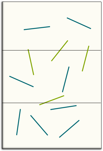
I’m not going to go into the details of why the experiment works. For the purpose of this article, what you need to take out of Numberphile’s video is the fact that, when thrown, a needle has a probability of $1/\pi$ to cross a line. Thus, in virtue of the law of large numbers, when a great number of needles are thrown, the ratio of the total number of needles divided by the number of needles crossing a line should approach $\pi$.
Hummm… $\pi$ has an infinite number of digits which cannot be represented on any known physical support. This includes our brains and the entire universe. Thus, I’m sorry to break it out, but we will never know $\pi$. At best, we can have a great approximation of it. Now, there are better ways than Buffon’s to obtain more accurate approximations. But, in this article, let’s imagine that Numberphile’s experiment is the best approximation of $\pi$ mankind has ever done.
No! We know precisely that the result isn’t… precise. In fact, $\pi$ has been proven to be irrational, which means that there is absolutely no hope that the experiment provides the exact value of $\pi$.
Of course not! And statistics will tell us just how meaningful the measure is!
Testing $\pi=3$
One framework provided by statistics is hypothesis testing. It seems so relevant to me that it’s the sort of reasonings I wish everyone knew about. Especially people whose minds are stubbornly made up!
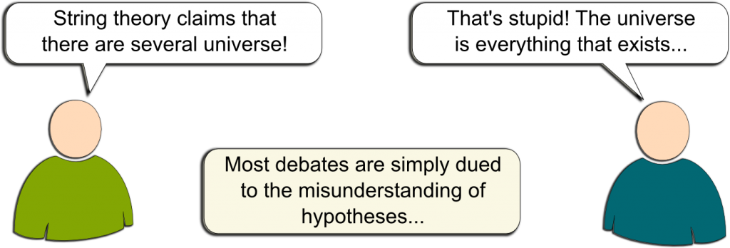
To test a hypothesis, we first need… a hypothesis! By hypothesis, I mean a statement we will be testing with the experiment. Requiring a hypothesis might sound obvious, but the mere effort of clearly stating hypotheses would magically solve most debates! More often than not, arguments originate from the misunderstanding of others’ hypotheses… if not the misunderstanding of one’s own hypothesis! For instance, relevant reasonings on multiverse theory often fall into deaf ears simply because of the ambiguity of the concept of universe:
Let’s consider the hypothesis $\pi=3$. This is the hypothesis to be tested. It’s thus commonly called the null hypothesis.
If all I knew was that $\pi$ was defined as the ratio of the circumference of a circle divided by its diameter, I’d bet $\pi$ to be a very simple number. And 3 is a simple number which isn’t too far from what was obtained by Tony Padilla. Plus, taking a hypothesis which is known to be wrong will highlight the misconception one might have about hypothesis testing.
Now, we turn our attention to the consistency of the experiment with the hypothesis.
Not necessarily. In fact, the hypothesis $\pi=3$ and the theory of probability predict that the result of the experiment will likely be $\pi \neq 3$. But they do also predict that, very likely, the result of the experiment should be close to $\pi=3$.
Precisely! At this point, what’s usually done is the use of the scientific method paradigm. According to this paradigm, a hypothesis is true until proven wrong. This means that, as long as the experiment doesn’t really falsify the hypothesis $\pi = 3$, this hypothesis needs to be assumed to be right.
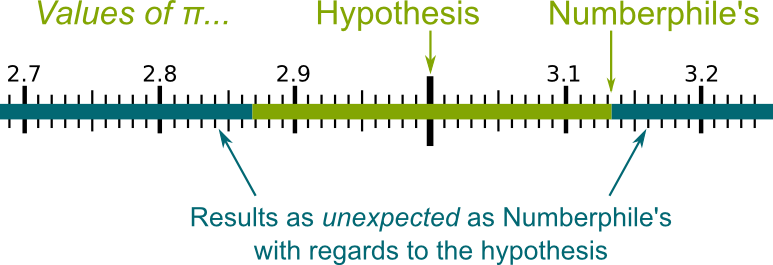
First, we need to consider all possible results which are at least as unexpected as the one obtained. In our case, the hypothesis says that we should obtain about $\pi = 3$. Thus, values as unexpected as Numberphile’s $\pi$ are those which are farther away from $\pi=3$ than Numberphile’s $\pi$. This is displayed the figure below:
What’s of even greater interest to us is the probability of these unexpected results. This is called the p-value. If the p-value is very low, then this means that the obtained result is extremely unlikely, according to the theory. In such a case, we reject the hypothesis.
Scientists usually consider the 5% rule! If you consider a higher threshold such as 10%, then, 10% of the time, you will reject hypotheses when they are actually right. On the other hand, small thresholds guarantee that you’ll hardly ever reject right hypotheses. The drawback is that you risk to often accept hypotheses even when they are wrong. In particle physics, where truth is the Holy Grail and we want to make sure we don’t reject right hypotheses, a very small threshold is used. This threshold is often about 10-7, which corresponds to the 5-sigma rule you might have heard about regarding the Higgs boson. We’ll discuss it in more details later.
Since we don’t have that much data, let’s consider a large threshold like 10%. This will give us more chance to reject the hypothesis… Even though it also leaves us with a greater chance to make a wrong rejection, which would correspond to a false positive!
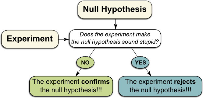
Sure! The general idea of hypothesis testing is depicted on the right. All we are left with is now computing the p-value, and then comparing it with our threshold of 10%. To do so, we’ll need a little bit of probability theory…
Computing the p-value
In the 19th Century, Karl Friedrich Gauss, one of the greatest mathematician of all times, noticed a recurrent pattern in Nature. Measurements often displayed a certain distribution, known as normal distribution, Gaussian distribution or bell curve.
This distribution appears, for instance, in the following wonderful experiment by James Grime at Cambridge science festival 2013:
Yes! And this video illustrates a very strong mathematical result of probability theory: The bell curve appears when we add up random variables. In James Grime’s experiment, at each stage, balls either go left or right. This corresponds to adding 1 or -1 to their x-axis. Over all stages, the eventual x-coordinate of a ball is the sum of variables equalling randomly either 1 or -1. The central-limit theorem states that such sums are random numbers which are nearly distributed accordingly to a bell curve.
The number of needles crossing a line is the sum of random variables!
Yes! Each needle can be associated with a number: 1 if it crosses a line, and 0 otherwise. Such numbers are called Bernouilli random variables. The number of crossing needles is then obtained by adding all these numbers for all needles!
We can thus apply the central-limit theorem to assert that this number of crossing needles is nearly distributed accordingly to the bell curve.
This means that this number of crossing needles can be regarded as random variable, which would take other values if we redid the experiment. And if we redid experiments over and over, the numbers of crossing needles of these experiments would nearly have a bell curve distribution, just like balls were in James Grime’s experiment.
We’re getting there! Bell curves depend on two parameters. First is the means. It’s the average number of crossing needles. Since, each needle has a probability of $1/\pi$ to cross a line, the average number of crossing needles is $N_{total}/\pi$. If our hypothesis $\pi=3$ is right, then this average number is $N_{total}/\pi = 163/3 \approx 54$. This means that the bell curve will be centered around the value 54.
The second parameter is the variance. It basically says how much variation there is from one experiment to another. An important mathematical property of the variance is that the variance of the sum of independent random variables is the sum of the variance of each random variable. Thus, in our case, the variance of the number of crossing needles is 163 times the variance of the Bernouilli random variable associated to one needle.
Let me save you from the technical detail of this calculation and give you the result: $(\pi-1)/\pi$. Thus, the variance of the number of crossing needles is $163(\pi-1)/\pi$. Since $\pi=3$ according to our null hypothesis, this variance equals 163 x 2/3 ≈ 109.
The variance is the average square of the distance between two measurements. What’s more understandable is thus rather the square root of the variance, known as the standard deviation. It represents more or less the average distance between two measurements. In our case, it’s about $\sqrt{109} \approx 10$. This means that, in average, the number of crossing needles varies by about 10 between two experiments. Since Numberphile observed 53 crossing needles, anyone else doing the exact experiment should expect to obtain about 53, more or less about 10 needles. In other words, if you obtain 45, that’s perfectly normal. But if you obtain 85, then it’s very likely that something went wrong in your experiment (or in Numberphile’s).
Now, we can plot it! This gives us the following curve, where the height stands for the probability of measurement:
As you can see, obtaining about 45 is quite likely, but obtaining about 85 is very unlikely.
The values as unexpected as Numberphile’s with regards to the hypothesis $\pi=3$ are values greater than 3.13 or smaller than 2.87. Recalling that the measure of $\pi$ was obtained by $N_{total}/N_{crossing}$, I’ll let you prove that unexpected values correspond to $N_{crossing} \leq 163/3.13 = 52$ (this is what was found in the video) or $N_{crossing} \geq 163/2.87 \approx 57$. The cumulated probability of these two cases is the blue area below the curve depicted in the following figure:
After boring calculations I did for you, I’ve come up with the blue area, which is the p-value. It’s about 0.81. This means that obtaining values as unexpected as Numberphile’s with regards to the hypothesis $\pi=3$ is very likely. In other words, if $\pi=3$, then Numberphile’s result was largely to be expected.
Precisely! Even for our large threshold of 10%, Numberphile’s result provides an evidence that $\bf \pi=3$! Unfortunately, quite often, what I’m saying here is often rephrased as Numberphile’s result proving that $\pi=3$! I hope this shocks you. Now, have in mind that, for other more misunderstood claims, this is too often what’s said. Haven’t you read somewhere that genetics proved Darwin’s theory of evolution? Or that the Large Hadron Collider (LHC) proved the existence of the Higgs boson? Especially in mathematics, the word proof is sacred, and we absolutely avoid it when mere experimental measurements back up a hypothesis (except in articles like mine, precisely to point out its misuse…)!
As the scientific paradigm goes, tests are good to reject hypotheses, rather than confirming them! Albert Einstein once said: “No amount of experimentation can ever prove me right; a single experiment can prove me wrong”.
Fortunately, yes! And statistics is still up to the task to describe what is meant by more confirmed. This leads us to the concept of alternative hypothesis.
Alternative Hypothesis
Just like in real debates, to attack a hypothesis, one’d better be armed with an alternative hypothesis. In the case of the Higgs boson, the alternative of its existence of the Higgs boson is its non-existence. That was easy… Now, what’s the alternative of $\pi=3$?
That’s a bold assumption. I don’t see any reason why $\pi$ would take such a complicated arbitrary-looking value… But, why not?
What we have done so far was comparing the p-value with a threshold. As we’ve discussed earlier, this threshold stands for the probability, when the experiment is repeated, of rejecting the hypothesis when it’s actually right. This is known as the error of the first kind. Crucially, it’s often considered that we then accept the alternative hypothesis. So, the threshold on the p-value is the probability of accepting the alternative hypothesis when it’s actually wrong. In other words, it’s the probability of a false positive.
Yes! Namely, accepting the hypothesis when it’s actually wrong. More precisely, because we can’t do any reasoning without a hypothesis to build on, the error of the second kind is accepting the null hypothesis when the alternative is right. The following figure illustrates these two kinds of errors:
First, let’s see what measures reject $\pi=3$. A quick approximative computation I’m not boring with you shows that the null hypothesis gets rejected for less than 38 crossing needles or more than 71 ones. Indeed, the p-value of these measurements is about 10%. In other words, we accept the null hypothesis $\pi=3$ if the number of crossing needles is between 38 and 71.
Now, we need assume that the alternative hypothesis is true, namely that $\pi=3.14$, and compute the probability of mistakenly accepting the null hypothesis. Once again, I’m saving you from the unbearable details of computations. With the alternative hypothesis, the average number of crossing needles is now about 52, while the standard deviation is still about 10. The probability of accepting the null hypothesis is then the blue area of the following figure:
This blue area equals 0.87. This means that, in 87% of cases, the null hypothesis is mistakenly accepted!
No, it’s not. The thing is, there are just not enough data to tell the null hypothesis and the alternative one apart. This is why you can say that Numberphile’s experiment isn’t as convincing, as, say, LHC’s discovery of the Higgs boson, for which it was made sure that the probability of mistakenly accepting its existence was smaller than 10-7.
Yes! A spectacular other example of that is James Grime’s testing of the fact that the probability of living in an odd numbered house is 0.502: He rejected, with a sufficiently small probability of error, the alternative hypothesis according to which we’re equally likely to live in an odd numbered house or an even numbered one:
So what he really showed is that, with great confidence, we can say that we’re not equally likely to live in an odd or an even numbered house.
That’s an awesome question! Prior to any survey, this is the sort of question that has to be asked! It leads us to the concept of confidence interval.
Confidence Interval
The confidence interval is independent from any hypothesis. Rather, it detects the set of hypotheses which are consistent with experiment. This makes it very powerful.
First we need to choose a confidence level, which stands for the probability that the interval contains the real value of $\pi$. Let’s take this probability to be about 1-10-7. This probability corresponds to the 5-sigma rule we will see later on.
Now, we need to come up with a confidence interval constructed with the measure 52 of $N_{crossing}$ and the known parameters of the experiment like the total number of needles. Plus, and mainly, this confidence interval must contain the real $\pi$ with a great probability.
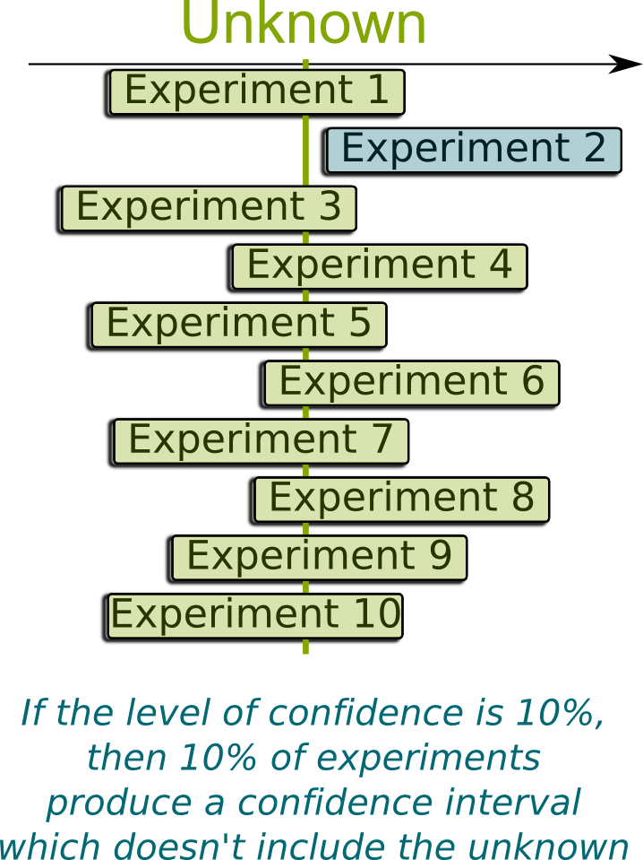
The real $\pi$ is a fixed number indeed. However, the confidence interval is built on the results of the experiments, which are random. Thus, the confidence interval is random! The probability I’m talking about is the probability that our constructed random confidence interval contains the fixed unknowns. In other words, if we redid the experiment over and over, we’d obtain plenty of different confidence intervals. We want nearly all of them to contain the real $\pi$.
We usually center it around the measured value $N_{crossing} = 52$. The 5-sigma rule then consists in including in the interval all values at less than 5 standard deviations from the measured value. Since the standard deviation was 10, this means that the confidence interval is nearly the interval $2 \leq N_{crossing} \leq 102$. This corresponds to values of $\pi$ in the interval $163/102 1.6 \leq \pi \leq 163/2$. With great confidence, we can thus assert that, according to Numberphile’s experiment, $\pi$ is somewhere between 1.6 and 83… Not that great, huh?
The key element is that, when we quadruple the number of needles, we’re quadrupling the average number of crossing needles as well as the variance. But since the standard deviation is the square root of the variance, we’re only doubling the standard deviation. In other words, with more and more needles, the average number of crossing needles grows much faster than the standard deviation. This enables us to narrow down the interval confidence around $\pi$.
Once again, I’ll save you from the flatness of computations. By having 60,000 needles, the average number of crossing needles will be about 19,000, while the standard deviation gets to around 200. This gives a width of the confidence interval on $\pi$ of about 2 x 5 x 200 / 19,000 ≈ 0.1. This is smaller than the distance between the two hypotheses $\pi=3.14$ and $\pi=3$. It will thus tell the two hypotheses apart!
You’d have to be 100 times more accurate, as you’ll have to tell apart the $\pi$’s 4th digit rather than only the 2nd. As often in statistics being 100 times more accurate requires 1002 more data. This amounts to 600 million needles! I’d love to see Numberphile undertaking that experiment!
Statistics still has an answer to this. Actually, several answers. The more straightforward one is the method of moments, but it fails to apply in more complex problems. In such problems, there’s the likelihood method. You can learn more on the likelihood method by reading about how I modeled football games!
Yes! The existence and non-existence of the Higgs boson implied a difference of a particular measurement. This difference is extremely small, which is the reason why billions of billions of particle collisions were required to tell the two hypotheses apart. After years of work, scientists at LHC have succeeded in obtaining sufficiently many data to conclude with confidence of about 1-10-7 that the Higgs boson couldn’t not exist. Which was then rephrased more or less correctly as scientists being 99.99994% sure of the existence of the Higgs boson. Rather, it means that if the experiment was done millions of times, only a few of them wouldn’t reject the non-existence of the Higgs boson.
That’s an awesome point. It’s essential! Einstein’s general relativity has convinced everyone because several experiments have aimed at discrediting it without success. In fact, a major illustration of the use of several tests is its application to probabilistic algorithms like face detection or quantum computing!
Let’s Conclude
Statistics is a wonderful field of mathematics with solid reasonings… on blurrier ones. It’s essential to uncover the apparently random and fuzzy patterns of Nature and human interactions. I’d claim that it’s only by getting statistics right that one can get his reasonings right in soft science. Unfortunately, reasonings with statistics often involve lots of calculations, and, even in this article, I feel like I’ve included too many of them. Yet, the philosophy behind is both calculation-free, extremely powerful and too often misunderstood. I wish more people mastered it better. It would solve so many debates…
Keep in mind that, using the popular scientific method, Numberphile’s experiment strongly confirms that $\bf \pi=3$. Indeed, this scientific method consists in rejecting ideas only once we are nearly sure that they are totally inconsistent with observations. This implies that it accepts or confirms many hypotheses even though they may be deeply wrong. Similarly, even when observations vindicate your ideas, these ideas may well still be awfully wrong. That’s part of the reason why I don’t like the scientific method. I know there’s more to it, but I still largely prefer Hawking’s model-dependent realism, or even a more drastic position assuming the inaccuracy of all theories (namely, instead of chasing the truth, let’s aim at good modelings of observations).
Exactly! In fact, Numberphile’s result is suspiciously close to the real value of $\pi$… as it was unlikely to be that close (an odd of 7%)! In comparison, the equivalent unlucky case would be to measure $\pi=4.8$! Not sure Tony Padilla would have been as happy with such measure. In fact, my suspicions lead to two possibilities: either Tony Padilla was extremely lucky, or his acting is state-of-the-art!
Finally, to come back to Johnson’s study, an interesting idea put forward is that the threshold of the p-value should depend on prior knowledge. For instance, if you want to confirm that gravity pulls, you may not need a small threshold. However, if you want to prove that your set-up made life appear out of nowhere, you’d better make sure this is not a statistical error! In this latter case, you should use a very small threshold of the p-value. Amusingly, physicists already apply such a concept as they require a 3$\sigma$ error for confirmations, but a 5$\sigma$ one for discoveries!




I think there is a reason for Tony Padilla’s luck :
His sampling is not totally random, since his needles never overlap. Therefore, he has a kind of Poisson Disk sampling, with skinny needle-shaped rectangles instead of disks:
http://devmag.org.za/img/articles/Poisson_Disk_Sampling-figure%201.jpg
As far as I know (I am not a pure mathematician but work with computer graphics, and rendering deals with a lot of statistics), Monte-Carlo methods converge faster with a smartly chosen sampling…
Great point!
But I’m not sure how to quantify that non-independence between matches mathematically, but it does lead to a decrease of the variance of the estimation. Now, even then, I’d still say that Tony Padilla was very lucky!
Great post.