Linear programs have an amazing structure. The simplex methods exploit this amazing structure to quickly find optima. Thanks to that, problems with millions of variables can now be solved, hence solving extremely complex industrial issues. That’s why the simplex methods have become crucial in our world today.
You’re right to ask. There really is only one simplex method, introduced by the American mathematician George Dantzig right after the second world war. However, variants have been introduced, mainly the dual simplex method, which I’ll present later in this article. Let’s have a look at the simplex method first.
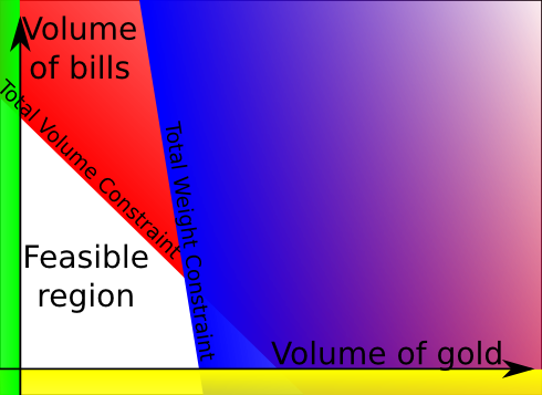
We’ll consider the smart robber problem I described in my article on linear programming, that is we can steal bills or gold, but the total stolen volume is limited, as well as the total weight stolen. Here is a figure of the feasible region.
The simplex method
Recall that, in a linear program, there is necessarily an extreme point that is the optimum.
There are two problems with listing all the extreme points. First, there can be a lot of them, especially when considering problems with millions of variables and hundreds of thousands constraints. Second, finding an extreme point can be quite difficult as it involves solving a system with all the constraints that may not lead to a feasible solution. Shortly said, listing all the extreme points is a bad idea.
What the simplex method does is moving from extreme points to strictly better extreme points until finding an optimal extreme points. This simple idea is considered as one of the main breakthroughs of the 20th century in computing, at least according to the journal Computing in Science and Engineering!
Any extreme point is the intersection of enough faces of the polyhedron. How many faces? As many as the dimension of the feasible set. Let’s call n this dimension. Be careful if you read other articles on linear programming, n may refer to something else like for instance the number of variables.
Now let’s notice that the faces of the polyhedron are the constraints. Thus, an extreme point is the intersection of n constraints. In our case, the feasible set is of dimension 2, so any extreme point is the intersection of at least 2 constraints.
Almost. Let’s define a constraint base as a set of n constraints.
It might seem like constraint bases can describe extreme points equivalently. Unfortunately, the relation between constraint bases and extreme points is not that simple for two reasons. First, a constraint base doesn’t necessarily describe an extreme point. For one thing, two constraints could totally match or be parallel and the intersection of n constraints could be empty or infinite. This is rare and could be dealt with. But, more importantly and more frequently, the intersection could be a point outside of the feasible set (like for instance the intersection of the red and yellow constraints of our example). Such constraint bases are called infeasible constraint base.
Another thing that can happen is that an extreme point could be described by several constraint bases. As a matter of fact, it’s possible that more than n constraints intersect at an extreme point. In this case, any constraint base describing this degenerated point is called a degenerated constraint base.
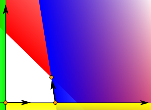
Still, despite these defaults, we use constraint bases to describe extreme points. Now, I’ll repeat what I said earlier about the simplex method but I’ll use constraint bases right now. At any extreme point, the simplex method seeks for a next feasible constraint base to visit, that is strictly better than the current constraint base. In order to do that, it looks at the possible direction where it can go to reach a next extreme point via an edge of the polyhedron. This direction is described by the constraint it will get out of the constraint base. The constraint base without one constraint gives a line to follow, delimited by our current extreme point. As we walk along the line, we eventually reach a new constraint that will enter the constraint base. This defines a new feasible extreme point.
There’s something else that’s particularly interesting with that method. Although computing an extreme point given its constraint base can be difficult for high dimensions (it requires the inversion of a matrix n x n), moving from one extreme point to a neighbor extreme point can be done very quickly. That’s one of the reasons why the simplex method is very efficient.
It knows by looking at the reduced cost associated with the direction. The reduced cost is how much the objective function will improve with one step in the given direction. It can be computed by making simple operations on the constant parameters of the linear program, or by looking at the dual variables. I’m not going to get into the computation of the reduced costs, as it’d be much more interesting if I had talked about those dual variables. Learn more by reading my article on duality in linear programming.
The following figure shows what the simplex method would do in our case:
Here’s a way to visualize the simplex method. Imagine that you hold the polyhedron in your hands. That’s your feasible set. Add pipes on every edge. Those pipes link extreme points of the polyhedron. Now, choose the inclination of the polyhedron. This inclination represents the objective function: the horizontal plane should be a level set, while the vertical should be the gradient (don’t mind about this word if you don’t know what it means). Now, what the simplex does is choosing a first extreme point, and inject a drop of water in it. Then the simplex will choose the path of the drop of water (providing it never divides) until reaching the lowest point of the polyhedron, which will be the optimal point.
As you can imagine, choosing a good starting extreme point is crucial for the speed of the algorithm. It’s better to have one close to the optimum. However, this is a difficult problem. In fact, even finding one extreme point is hard. We usually introduce another program to solve this problem: minimizing the non-feasibility of solutions. In this program called Phase I, every solution is feasible, and what’s particularly great, the program is a linear program… which therefore can be solved with a simplex method!
The simplex method has become famous and has been used a lot as it enabled the resolution of problems with millions of variables and hundreds of thousands of constraints in reasonable time. However, it faces problems in cases of degeneracy: it’s possible that the direction of the reduced cost points out of the polyhedron (and that actually happens very often when using column generation). It’s hard to anticipate whether a direction will point out of the polyhedron or not and testing all the directions can take quite a while.
Moreover, the performance of the simplex method is being questioned by the rise of interior point methods. Shortly said, interior point methods penalize points in the border of the feasible set and slowly decrease these penalties to converge to the optimal point. Interior point methods deserve their own article. If you know them, please write about them!
Because the research on simplex methods is still very productive, and many of its variants are state-of-the-art for specific problems. Let’s mention the column generation for shift scheduling, vehicle routing or clustering. This method is particularly developed in companies and universities in Montreal. It is used with the Dantzig-Wolfe decomposition. Shortly said, the idea is to consider only the vectors that may improve the objective function.
Stochastic programming enables to solve programs with probabilities very efficiently thanks to the L-Shaped method, derived from the Bender’s decomposition. The L-Shaped method can be understood as a method that only adds the constraints that are relevant, by detecting those that are not satisfied when not deleted.
Last but definitely no least, integer linear programming is very efficient using the simplex method! Integer linear programming enables modeling of a very very large range of fields that include binary variables for instance. Examples of these fields are assignment, supply chain and location problems. Find out more with my article on the topic!
All those methods correspond to exact methods (which means that they find the actual optimum). They may be too long. That’s why plenty of approximate methods, called heuristics, have been developed to find a point close to the optimum. These heuristics can be variant from the simplex.
Mainly because when we slightly modify a linear program, re-optimizing using the simplex method can be done very quickly, as we can start with an extreme point that will be close to one of the new extreme optimal points. In comparison, the interior point method cannot take information from the previous linear program resolution to solve a slightly modified linear program. This re-optimization will probably require the use of the dual simplex, which I’ll now introduce.
The dual simplex
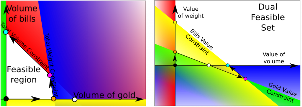
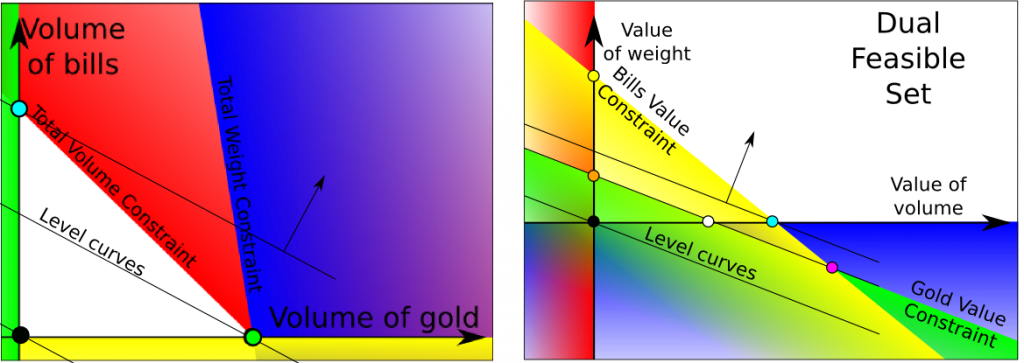
I’m now going to explain what’s happening in the dual as we apply the simplex method to the primal. This well help us define another way of solving linear programs, known as the dual simplex. In order to have interesting things to talk about, we’ll assume that the optimal solution is to steal bills only. This gives us the following primal-dual spaces.
As you can see on the graphs, primal and dual bases can be associated. The optimal primal-dual solutions are the cyan dots. Let’s have a look of a possible path taken by the simplex algorithm in the primal and dual spaces.
The black dot is the initial base solution. Recall that the simplex method will finish when we reach a dual feasible base. At the primal black dot, the primal reduced costs are positive both when leaving the yellow and green primal constraints. This corresponds to having the two violated dual yellow and green constraints. We need to choose one of the primal base variable with a positive reduced cost, which corresponds to choosing one of the two violated dual constraints. In our case, we have chosen the green constraint.
Now that we have chosen the primal green constraint to leave (and, equivalently, the dual green constraint to reach), we need to decide where to stop. In the primal space, we have to follow the yellow constraint until reaching a base. Equivalently we choose another feasible base with the yellow constraint. This corresponds to the primal orange dot, rather than the white dot. What does that correspond to in the dual? By getting the green constraint into the dual constraint base, we can choose to either lose the dual red constraint or the dual blue constraint (one of the constraints that was already in the dual constraint base). The one we have to choose, in order to have it corresponding to the primal base, is the one with the worst better dual value (since we have a dual minimization problem, it’s the smallest higher dual value). As a result, we need to choose the orange dot.
We must choose the worst better dual value because we need to keep the dual reduced costs positive (if the dual program is a minimization program), so that when we reach a feasible dual base, we’ll be at the optimum for sure.
Each pivot in the dual space should be done as the one we just did. From the dual orange dot, only the dual yellow constraint isn’t valid, so we have to get it into the dual constraint base, which leads us to choose the worst dual value between the yellow and pink dots. The pink dot has a worse dual value, so we pivot towards it.
Then, from the dual pink dot, only the blue constraint isn’t satisfied, so we’ll get it into the dual constraint base. We then have to choose between the cyan and the white dots, but, as the white dot has a worse dual value, we cannot go there. So we’ll go to the cyan dot. The cyan dot is feasible, thus it is the dual optimum.
Well, it is useful for our understanding of the primal simplex. But that’s not all. The dual simplex is very useful if our initial point is non-feasible, in which case the primal simplex is useless (and we actually need to solve a subproblem called phase I, in order to find a feasible primal point). Yet, having an initial non-feasible point happens very very often in case of integer programming or stochastic programming using Bender’s decomposition. In both cases, we actually add new constraints to the primal linear program that make our current base infeasible. We can therefore apply the dual simplex to re-optimize. What’s more the dual simplex will perform very quickly as the initial base, which is usually the optimum without the new constraints, is very likely to be close to the new optimum.
The dual simplex is actually the reason why the variants of the simplex method work better than the interior point method on several important classes of problems.
Degeneracy
Just like for the primal simplex, the dual simplex performs well in case of non-degeneracy. However, if the primal simplex reaches a degenerated point, it may have a lot of trouble to get out of it because of the many bases that can represent the degenerated point.
Let’s draw this out to find the answer.
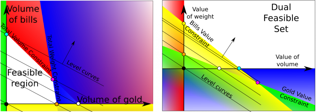
Just like in my article on duality, we moved the primal blue constraint to create a primal degenerated solution. As a result, the primal green dot is actually the merging of the primal orange, white and pink dots. Yet, moving a primal constraint does not affect dual constraints. It does, however, modify the dual objective function, thus the level curves.
Since the orange, white and pink primal base correspond to the same point, their have the same objective value, which implies that dual orange, white and pink dots are on the same dual level curve. The degenerated primal point could actually be associated with the dual polyhedron defined by the convex hull of the three dual dots. This concept of dual polyhedron is very important for column generation.
In our case, things remain simple because there is no much degeneracy and the dimension is very low. Thus, the path we used earlier is still valid and is actually the one taken. What’s more, the dual polyhedron associated with the degenerated point is very simple since it’s a line with three bases. However, in case of more degeneracy and higher dimension, the dual polyhedron could be enormous, and the dual simplex would be travelling all over the dual polyhedron. It may take a very long time for us to leave this dual polyhedron.
It’s important to notice that a primal degenerated pivot (that is, a modification of the base that does not modify the associated solution) corresponds to an actual dual pivot that does not improve the objective value. In cases of higher dimension and higher degeneracy the number of such pivots could be exponential. That’s where comes the idea of dual variable stabilization.
Let’s sum up
The simplex methods are amazing methods that exploit the structure of linear programs. In order to solve even larger problems, a better management of the bases must be done. That’s where technics like column generation and Bender’s decomposition are used and very efficient. However, they may be slow in cases of degeneracy which actually are very common in many classical modelings. Other technics are being developed to deal with degeneracy including the dual variable stabilization (read this article of mine) or the improved primal simplex.
Overall, the main application of linear programs concerns integer linear programming, which can model a very large range of problems. Many additional technics need to be added though, including the branch and bound, the cutting plane method, or, more recently, the integer simplex. Much research still needs to be done to improve integer linear programming.


